Bayesian estimation of a power law process with incomplete data

HU Junming, HUANG Hongzhong, and LI Yanfeng

1. School of Mechanical and Electrical Engineering, University of Electronic Science and Technology of China, Chengdu 611731,China; 2. School of Transportation and Automotive Engineering, Xihua University, Chengdu 610039, China; 3. Center for System Reliability and Safety, University of Electronic Science and Technology of China, Chengdu 611731, China

Abstract: Due to the simplicity and flexibility of the power law process, it is widely used to model the failures of repairable systems. Although statistical inference on the parameters of the power law process has been well developed, numerous studies largely depend on complete failure data. A few methods on incomplete data are reported to process such data, but they are limited to their specific cases, especially to that where missing data occur at the early stage of the failures. No framework to handle generic scenarios is available. To overcome this problem,from the point of view of order statistics, the statistical inference of the power law process with incomplete data is established in this paper. The theoretical derivation is carried out and the case studies demonstrate and verify the proposed method. Order statistics offer an alternative to the statistical inference of the power law process with incomplete data as they can reformulate current studies on the left censored failure data and interval censored data in a unified framework. The results show that the proposed method has more flexibility and more applicability.

Keywords: incomplete data, power law process, Bayesian inference, order statistics, repairable system.

1. Introduction

Reliability is a crucial characteristic for products because their higher reliability always leads to less loss and greater competitiveness. Many efforts have been made to meet expected specifications of product reliability in practice[1]. For example, the reliability growth management incorporates corrective measures to fix the defects that have surfaced and the reliability is enhanced gradually by the implementation of the test–analysis–fix–test cycle for product prototypes [2]. In addition to the reliability growth,sound maintenance policies and procedures also help to ensure that product reliability is maintained at the benchmark level after it comes into the operation. For both reliability growth and maintenance, failure data collection and analysis are the primary concerns [3]. Over the past decades, multiple approaches like Bayesian network [4-6], renewal process [7], trend-renewal process [8,9], Markov process [10-12], nonhomogeneous Poisson process [13-15], and modulated power law process [16], have been proposed to help analysts to make informed decisions.

Although there are different models, the power law process (PLP) is commonly used for failure data analysis due to its flexibility and ease of use. After the Army Materiel Systems Analysis Activity initially uses it to plan,track, and project a reliability growth program [17], the International Electrotechnical Commission recommends it for reliability growth modeling [18]. Moreover, the PLP is not restricted to dealing with data produced by the improvement program and is also suitable for handling data from other scenarios such as minimal repairs [19].Although the procedures that deal with parameters estimation, confidence intervals, prediction intervals, and the goodness-of-fit test of the PLP have been well established [20], the PLP still attracts much attention. Multiple investigations—the PLP model selection taking into account system heterogeneities [21], Bayesian inference of the PLP under different maintenance policies [22], statistical inference of the PLP considering competing risk[23], the generalized confidence interval of the scale parameter [24], conjugate prior for Bayesian inference of the PLP [25], and parametric bootstrap confidence interval method [26]—have been conducted.

Most of the literature use the PLP to perform the data analysis, which assumes that the failure times are fully known, that is to say, the successive failure times of the repairable systems are monitored and accurately recorded.However, failure data may not be detected or obtained due to various uncontrollable reasons. For example, human error, lack of experience, and malfunction of sensors may trigger any unobserved or unrecorded failure. Sometimes, the data may be found to be unfaithful or even incorrect. In practice, it often occurs that the exact failure times are not recorded and that only the number of failures occurred within a given period is known. Incomplete data can reduce the representativeness of the data sample and result in a distorted inference in turn [27].The interest in the incomplete data problem is therefore growing. Guo et al. [28] proposed a three-parameter Weibull failure rate for the analysis of incomplete wind turbine failure data, where a new time parameter was introduced into the Weibull rate function to represent the past running time.

Statistical inferences of incomplete data have also been discussed for the PLP. Yu et al. [29] carried out a statistical inference and prediction analysis of the PLP with left censored data by using the classical approach in which the missing data occurred at the early stage of the research. This work laid the groundwork for further studies.Based on the obtained results, Tian et al. [30] established Bayesian estimation and prediction of the PLP with left censored data; Chumnaul and Sepehrifar [31] derived a generalized confidence interval for the scale parameter of the PLP with left censored failure data; Na and Chang[32] conducted a trend analysis for tank maintenance where the left censored data are from multiple machines and no information on the number of missing data is available. Besides, some researchers have performed reliability studies that are subject to interval censored data.For example, Taghipour and Banjevic [33] conducted a trend analysis of the PLP with interval censored data.Peng et al. [34] suggested a framework to evaluate the dynamic reliability of repairable systems with interval censored failure data in which the imputation method was used to fill out missing data.

The above-mentioned methods deal with incomplete data based on their respective assumptions. They are limited to their specific cases, either left censored data or interval censored data, and no unified framework is available for handling all situations. In addition, the suggested methods are complex and lack flexibility since the successive failure times of the PLP are mutually dependent. Considering that order statistics can help manipulate the dependent variables into independent variables, it can provide an alternative viewpoint for dealing with missing data and simplify the related mathematical derivations. This paper proposes a generic approach for making statistical inferences of the PLP with incomplete data.

The rest of the paper is organized as follows. Section 2 introduces the preliminaries on order statistics and the PLP. After the likelihood function of the observed data is derived from the perspective of order statistics, Bayesian procedures of estimating unknown parameters of the PLP are discussed in Section 3. Section 4 provides case studies to explain and validate the proposed process, where both simulated and actual failure data are used. Finally,Section 5 summarizes the conclusions of this study.

2. Preliminaries

In this section, we briefly review some basic properties that are necessary for later discussion and mathematical derivation.

2.1 Order statistics

Given any random variable X1,X2,···,Xn, the i th order statistic, Xi:n(i=1,2,···,n), is defined by sorting the corascending order as X1:n≤X2:n≤···≤Xn:n.responding realizations of these random variables in an

When the random variable X1,X2,···,Xnis sampled from the same population, its realization x1,x2,···,xnis independent and identically distributed. Let f(x) andF(x)be the associated probability density function (PDF) and cumulative distribution function (CDF). The joint PDF of x1,x2,···,xnis equal toFurther, there are n! permutations of X1:n,X2:n,···,Xn:nto generate the same sample,i.e., each of these permutations has an equal chance of being the same order statistics. Thus, there is an n! to one map from the observations to the order statistics. The joint PDF of order statistics X1:n,X2:n,···,Xn:nis

where n! is the factorial of n.

For any two order statistics Xi:nand Xj:n(1 ≤i ＜j ≤n),the joint PDF of Xi:nand Xj:nis given without proof as

More details about (2) can be referred to [35]. Three identities, which are related to the derivation of (2) and also useful for further theoretical development, are described as follows:

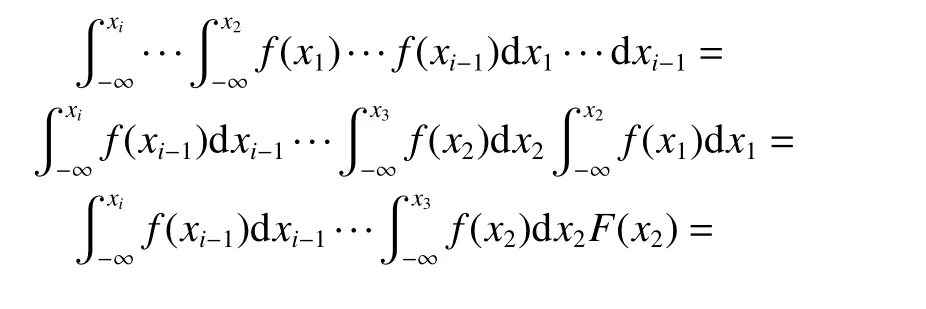
By integration of order statistics over their domain, (3)can be easily derived. Similarly, there exist

and

2.2 Power law process

The PLP is a nonhomogeneous Poisson process with a time-dependent failure intensity that is proportional to a power of time t. Let α and β denote the scale parameter and shape parameter separately. The failure intensity of the PLP, ν (t), is

Because the failure intensity of the PLP has the same form as the failure rate of Weibull distribution, the PLP is also known as the Weibull process [36]. If β ＞1, the system is deteriorating. If β ＜1, the system reliability is improving. If β=1, the system has a constant failure intensity and the PLP reduces to a homogeneous Poisson process.

The mean value function m(t) of the PLP is

where N(t) denotes the number of failures observed up to time t. Furthermore, according to the property of the nonhomogeneous Poisson process [37], the probability of N(t)=nis

Let T=(T1,T2,···,Tn) denote the consecutive failure times of a PLP where Tiis the i th failure time, tcis the time at which the data collection ceases. In practice, there are two types of truncated data: failure truncated and time truncated. If the data collection process is ceased at the arrival time of the nth failure, the data collected in this way are failure truncated. If the data collection process is terminated at a prefixed time, the collected data are called time truncated data. Thus, for failure truncated case, tcis equal to tn, and for the time truncated case, tcis predetermined.

Given the truncated time tcand the observed values T1=t1,T2=t2,···,Tn=tn, the joint PDF is

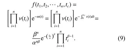
The conditional density function of T=(T1,T2,···,Tn)given N(tc)=n is

Equation (10) indicates that on the condition of N(tc)=n, the successive failure times T =(T1,T2,···,Tn) are distributed as order statistics from the distribution with PDF as

and the corresponding CDF is

Equation (12) shows that for the time truncated case,the successive failure data are that of n order statistics;while for the failure truncated case, the successive failure data are that of n−1 order statistics.

3. Analysis of incomplete data

To deal with the incomplete data, a unified framework combining the expectation maximization algorithm and Bayesian inference is proposed in this section.

3.1 Incomplete data

Incomplete failure data are common for repairable systems in practical situations. Different missing locations lead to different incompleteness forms. In this paper, the failure data are classified into two types: complete data and incomplete data. All failures are gathered and recorded for complete data. On the other hand, failure data in which certain elements are missing are classified into incomplete data.

Three types of failure data, complete data, left censored data, and interval censored data are shown in Fig. 1,where the symbol × stands for a failure and tiis the ith failure time. If the failure time is unrecorded, a subscript∗is used for indication. For both complete data and incomplete data, tcis the truncated time.

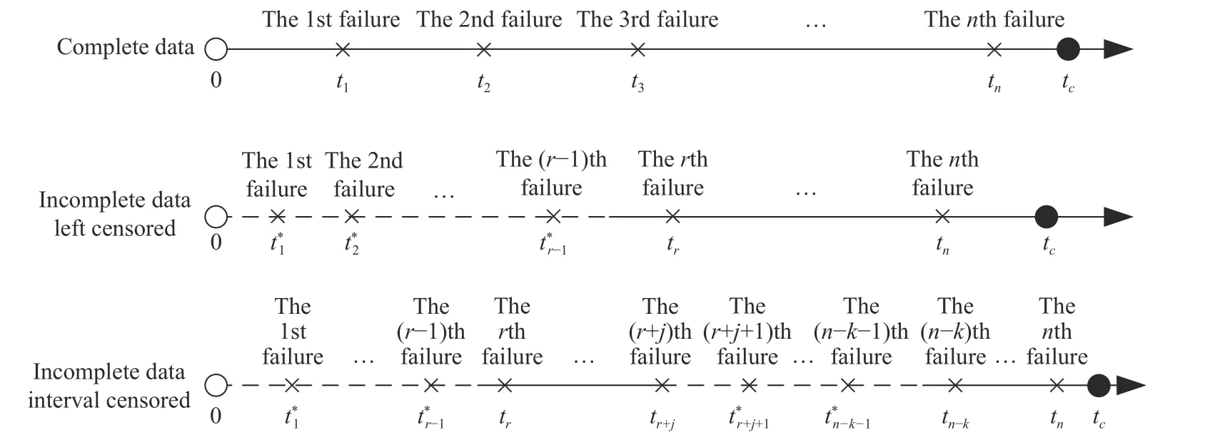
Fig. 1 Schematics of failure data

When the missing location is at the early stage, we term the data collected as left censored data. For example,the first r −1(1 ≤r ＜n) failures are assumed missing in Fig. 1, so the missing data are denoted byand the observed data are Yo={t1,···,tn}. If the missing occurs at certain periods, the data collected are regarded as interval censored data. For interval censored data in Fig. 1,the failures occurring at the interval (0,tr] and [tr+j,tn−k]are assumed missing. Thus, the missing data are denoted byand the observed data are denoted as Yo={tr,···,tr+j,tn−k,···,tn}.

3.2 Likelihood function

Dempster et al. [38] first presented a general approach to maximize the likelihood estimation of parameters with incomplete data. This approach assumes that there is a many-one mapping from the complete data to the incomplete data. Let the observed data and the missing data be denoted by Yoand Ymrespectively. The likelihood of complete data f(Yo,Ym|α,β) is related to the likelihood of incomplete data f(Yo|α,β) by

3.2.1 Likelihood of left censored data

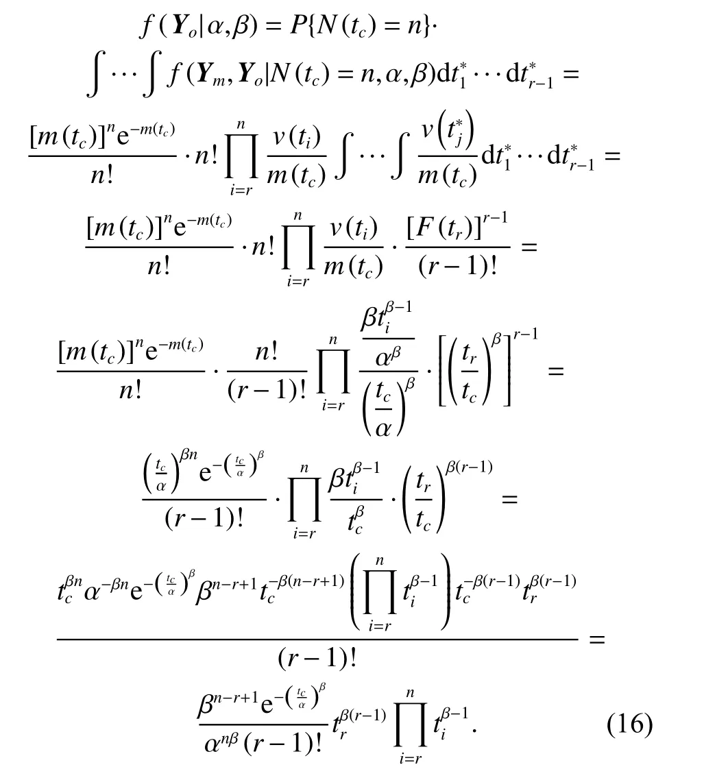
For left censored data shown in Fig. 1,and Yo={tr,···,tc}. The likelihood of Yocan be derived by integrating (13) with respect toi.e.,

As proofed in Section 2, the failure times of PLP are order statistics conditioning on N(tc=n) and its associated PDF and CDF are given in (11) and (12), respectively. Taking advantage of (2) and (3), and substituting(8) and (10) into (14), we can easily integrate (14) with respect to everyand obtain the likelihood of Yoas

Equation (16) provides a mathematical proof of (15).

3.2.2 Likelihood of interval censored data

Similarly, for the interval-censored case whereYm=and Yo={tr,···,tr+j,tn−k,···,tn},we can obtain the likelihood of Yoas

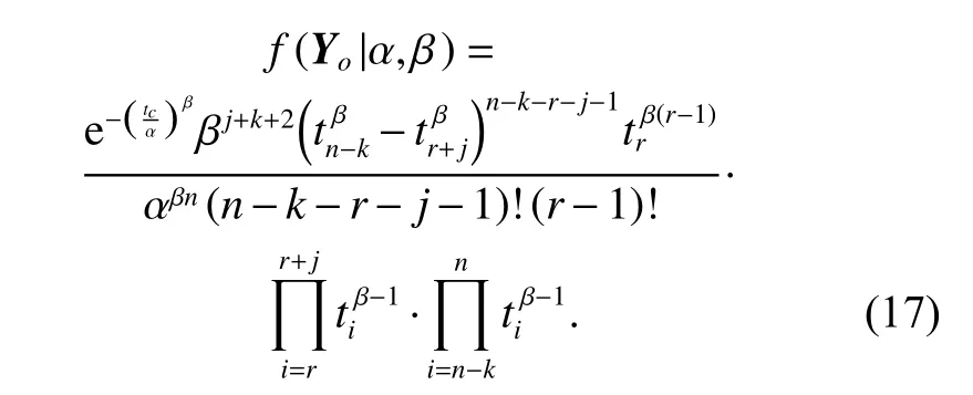
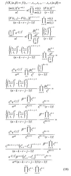
The mathematical proof of (17) can be referred to (18).

3.3 Bayesian inference

The Bayesian inference provides a useful approach to estimate unknown parameters in which the prior information and likelihood information are fused and more reasonable information on the unknown parameters can be yielded from the posterior. Let S stand for the observed data and P be the unknown parameters of interest. Under the Bayesian framework, the parameters P are assumed to be random variables. Assuming the associated prior PDF of P is f(P) and the likelihood function of S conditional on P is L(S|P), the posterior PDF of P , f(P|S), is determined by

The denominator of (19) is a normalizing constant. By this mechanism, the prior information f(P) is updated to the posterior f(P|S).

For the PLP, the scale parameter α and shape parameter βare the parameters of interest, i.e., P=(α,β). If α and βare independent mutually, f(P) is equal to f(α)f(β).The likelihood function of the observed failure data is determined by the failure data type. For complete failure data, L(S|P) has the form of (9). For the left-censored data, L(S|P) is defined by (15), and for the interval censored data, L (S|P) is given in (17).

4. Case study

In this section, we utilize two examples to illustrate and validate the proposed method. In the simulation case, all the data are generated in the same simulation. The Bayesian inference for the complete data, left censored data and interval censored data are conducted, and the inference results are compared. In the engineering case, real failure data from a reliability growth testing of a prototype vehicle are analyzed.

4.1 Simulation case

According to (10), the successive failure data of the PLP can be viewed as ordered statistics with the PDF and CDF as (11) and (12). This property provides a mechanism to simulate the PLP. For a time truncated case, simulation procedures for failure data are listed in Table 1.

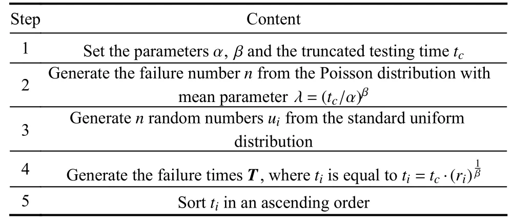
Table 1 PLP simulation procedures

A total of 27 failure times are simulated based on the procedures listed in Table 1, where the parameters α=50 , β=0.6, and tc=104. The successive failure times simulated are 4.4*, 29.8*, 104.4*, 217.8*, 656.1, 657.3,925.9, 1 624.8, 1 717.1, 2 043.0, 2 509.4*, 2 524.4*,2 664.8, 3 470.6, 3 673.4, 3 776.1, 4 599.9, 4 931.4,5 431.5, 5 437.2, 5 609.5, 6 532.4, 8 202.6, 8 398.9,9 154.4, 9 380.7, 9 969.6. Both the left censored and interval censored data are considered in this study. For the left censored data, the exact failure times for the first four failures are assumed unknown and are indicated by *.That is, n=27 and r=5 for the left censored case. For the interval censored case, additional failure times are assumed missing besides the first four failures times. All the missing data are denoted by *. That is, n=27,r=5 , j=5, and k=14 for the interval censored case.

Under the Bayesian framework, the prior knowledge,such as statistical data, expert opinions, historical data, or experiences from similar systems, can help to create a reasonable prior distribution. Prior elicitation, however,requires significant effort. Therefore, for the unknown parameters α and β in this study, noninformative prior distributions characterized by uniform distributions are adopted.

To verify and compare the effency of the proposed approach, all the cases use the same noninformative prior distributions where α and β are considered to be mutually independent. Using the Markov chain Monte Carlo(MCMC) sampling, the point estimation and 95% credible intervals are easily obtained from the posterior distribution. The results of the Bayesian inference are listed in Table 2.

Table 2 Inference results of different data types

As shown in Table 2, the point estimates of α andβ are similar to each other, and all the point estimates ofβ are very close to the actual value. The estimate thus captures the characterization of the system. In addition, all the credible intervals of α and β are valid. There is no significant difference between circumstances. It is verified that the proposed method is effective.

4.2 Engineering case

Two engineering cases from an aircraft generator and a prototype vehicle are used to illustrate the proposed methodology. For the first example, Chumnaul and Sepehrifar [31] gave the maximum likelihood estimates(MLE), classical confidence intervals (CCI), and generalized confidence intervals (GCI) derived from generalized pivotal quantity. The same data are used here for the comparative analysis. For the prototype vehicle data, we focus on determining whether the system is improving.

4.2.1 Aircraft generator data

The testing of an aircraft generator is ceased at the 13th failure. The observed failure data are 55*, 166*, 205*,341, 488, 567, 731, 1 308, 2 050, 2 453, 3 115, 4 017, and 4 596. For comparative purposes, a mathematical transformation γ=α−βis performed for consistency, so the failure intensity reduces to ν(t)=γβtβ−1and the parameters of interest in this case are γ and β.

We assume r=1 , 2, 3, 4, where r −1 is the number of missing failures at the early stage of testing. Similar to the left censored data of Subsection 4.1, the noninformative prior and the MCMC algorithm are used. The point estimates and credible intervals obtained are tabulated in Table 3, where the MLE, CCI and GCI provided by Chumnaul and Sepehrifar [31] are also listed.

Table 3 Parameter interval estimates for complete ( r=1) data and incomplete ( r ≥2) data

When the performances of interval estimates are compared, the interval widths obtained from GCI and CCI increase as r increases, and CCI has a bigger width than GCI. However, all the widths of credible intervals are closed to each other and are less than CCI and GCI. It indicates that the proposed method can yields precise results.

4.2.2 Prototype vehicle data

Reliability growth is an effective way to improve the system reliability. The failure data analysis can help identify whether the fixes are effective and the reliability is improving. A reliability growth testing for a prototype vehicle has been conducted where some potential failure modes are surfaced and corrective actions are incorporated.However, the exact failure data of the initial testing stage are not documented, and only the failure number is reported. The exact failure times recorded are 673.6, 697.4,796.1, 892.7, 906.3, 967.2, 1 066, 1 108. What is more,the exact failure times for the first 16 failures are not recorded, and the testing is terminated at 1 200 k.

To assess the reliability of the system after this stage of testing, the PLP is used to fit the data. Obviously, the data is the left censored type. Using the above methods, the marginal posterior distribution of β is obtained as shown in Fig. 2. The posterior mean of β is 0.65, with a 95%credible interval of (0.37, 1.14). The probability that β is less than one is quite large. It implies that the failure rate decreases over time. Therefore, the system performance is improved and the fixes implemented are effective.

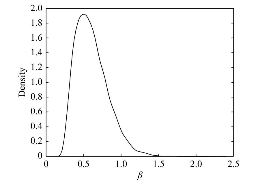
Fig. 2 Marginal posterior density of β

Similarly, it can be derived that the posterior mean ofα is 15.77, with a 95% credible interval of (0.15,78.71).Taking advantage of the inference results of α and β, the system reliability can be tracked and the present or potential level of reliability can be measured.

5. Conclusions

This paper develops a method for statistical inference of the PLP with incomplete data from the viewpoint of order statistics. It extends the application scenarios of the PLP because it can not only handle the left censored failure data, but also can be used for interval censored failure data. The mathematical derivation is comprehensive,and the case studies demonstrate and validate the effency of this approach.

Further research may focus on developing frequentist approaches for the interval censored case since frequentist approaches provide alternatives to Bayesian inference.For the parameters of interest, closed expressions on maximization likelihood estimators, confidence intervals,and prediction intervals can also be obtained from the point of view of order statistics. In addition, since the order statistics can simplify the successive failure times that are mutually dependent to be independent identically distributed, other methods such as the bootstrap approach and the Monte Carlo expectation maximization algorithm are also worth being studied for the incomplete data analysis. Comparative studies between different approaches are also required.

It should be noted that the incomplete data analyzed in this paper are limited to the situation where the exact time for failure is missing but the number of failures is known.Further research should pay attention to the situation where both the failure number and failure times are missed.

Acknowledgment

The authors extend sincere gratitude to the Technology Institute of Armored Force for the data provided.