Constrained voting extreme learning machine and its application

MIN Mengcan, CHEN Xiaofang, and XIE Yongfang

School of Automation, Central South University, Changsha 410083, China

Abstract: Extreme learning machine (ELM) has been proved to be an effective pattern classification and regression learning mechanism by researchers. However, its good performance is based on a large number of hidden layer nodes. With the increase of the nodes in the hidden layers, the computation cost is greatly increased. In this paper, we propose a novel algorithm,named constrained voting extreme learning machine (CV-ELM).Compared with the traditional ELM, the CV-ELM determines the input weight and bias based on the differences of between-class samples. At the same time, to improve the accuracy of the proposed method, the voting selection is introduced. The proposed method is evaluated on public benchmark datasets. The experimental results show that the proposed algorithm is superior to the original ELM algorithm. Further, we apply the CV-ELM to the classification of superheat degree (SD) state in the aluminum electrolysis industry, and the recognition accuracy rate reaches 87.4%, and the experimental results demonstrate that the proposed method is more robust than the existing state-of-the-art identification methods.

Keywords: extreme learning machine (ELM), majority voting,ensemble method, sample based learning, superheat degree(SD).

1. Introduction

In the past few years, many neural network architectures have been developed. Among them, single hidden layer feedforward networks (SLFNs) have been widely applied to various fields due to the advantages of simple structure and fast training speed [1]. The common method for training SLFNs is the gradient based learning methodback propagation (BP) algorithm [2], which updates the weight and bias of the neuron nodes by calculating the gradient of the loss function, so as to obtain a better network structure. However, the gradient based learning method has the disadvantage of slow learning speed and falling into a local optimal value. Although some improved methods have been proposed, such as Levenberg-Marquardt [3], evolutionary algorithm [4] and dynamic network construction [5], these algorithms still have high computational costs and cannot get the global optimal solution. The support vector machine (SVM), which optimizes the objective function based on the structural risk minimization, is one of the most popular algorithms for training SLFNs [6,7]. With the deepening of the research,it is found that the SVM algorithm is difficult to implement for large-scale training samples, and it is also difficult to solve multi-classification problems.

In recent years, the extreme learning machine (ELM) is proposed by Huang et al. [8] to train the SLFN. The ELM randomly generates the weights connecting the input layer to the hidden layer and the bias of the hidden layer neurons, and does not require any adjustment during the training process. Only by setting the appropriate number of hidden layer nodes, the optimal output weight can be obtained by constructing the least squares problem.Therefore, compared with the traditional methods, the ELM has the advantages of fast learning speed and good generalization performance. Recently, scholars have done a lot of researches on the ELM. Zhang et al. [9] proposed the incremental ELM based on the embedded deep feature, and the method performed well in classification.Ding et al. [10] used an auto-encoder to set the orthogonal weights and orthogonal thresholds of the ELM hidden layer, combined the unsupervised learning method with the ELM, and proposed a novel clustering algorithm. In view of the limitations of the traditional SVM regression prediction algorithm and the generalized neural network prediction algorithm, Wang et al. [11] combined cloud computing and the ELM for distributed power load forecasting. Experimental results show that the proposed algorithm has excellent parallel performance. Zhu et al.[12] proposed a short-term wind speed forecast method based on the ELM, which required shorter computation time than the traditional methods. Pan et al. [13] introduced the ELM into the reservoir permeability prediction and compared it with the SVM, the research results showed that the ELM has a higher prediction accuracy and more obvious advantages than the SVM in learning speed.Zhao et al. [14] used the convolution neural network to extract the multi-layer features from mammograms, then used the ELM to diagnose the breast diseases based on the fusion features, and the proposed method effectively improved the accuracy of the breast disease diagnosis.

However, randomly selecting the number of hidden layer nodes of the ELM according to artificial experience will affect the performance of the network. In particular application, the appropriate number of hidden layer nodes is usually in a relatively small range, in which the number of selected nodes has a small impact on network performance. When the number of hidden layer nodes is set too small, the network cannot reach the expected performance. When the number of hidden layer nodes is set too large, it will take a lot of time to train the network model,and it is also prone to over-fitting. Therefore, the random selection of hidden layer parameters will make the use efficiency of some nodes very low, resulting in structural redundancy [15-18].

In the ELM, the essence of the input layer to the hidden layer is to map the sample data from one space to another feature space, and then classify it in the output layer with a linear classifier [19]. However, because the learning parameters of the hidden layer are randomly selected,some samples close to the classification boundary may be misclassified. In order to reduce the influence of hidden layer learning parameters and reduce the number of misclassified samples, we improve the original ELM and a novel algorithm named constrained voting ELM (CVELM) is proposed. The proposed method uses the difference of between-class samples to form a difference vector set, and calculates the weight of the input layer to the hidden layer and the bias of the hidden layer according to the randomly selected difference vector. Multiple independent extreme learning machines are constructed for integrated learning, and the majority voting method is used to make decisions [20].

The main contributions of this paper are as follows:

(i) According to the difference vector composed of between-class samples, the weight vector between the input layer and the hidden layer is calculated, so as to avoid the influence of the random selection of hidden layer parameters on network performance.

(ii) The proposed method combines multiple independent ELMs and introduces a majority voting method for decision making.

(iii) The CV-ELM can greatly improve the accuracy for superheat degree (SD) identification, and the accuracy of the experimental result is as high as 87.4%.

The remaining of this paper is organized as follows.Section 2 introduces the basic ELM and gives the relevant theoretical knowledge of the constructing CV-ELM.In Section 3, we introduce the proposed CV-ELM algorithm. The experimental results of the public datasets and the SD state classification results in the aluminum electrolysis industrial process are presented in Section 4.Conclusions are drawn in Section 5.

2. Related works

In this section, we first introduce the basic ELM, then explain the selection of hidden layer parameters of the proposed method, and finally introduce the majority voting method.

2.1 Extreme learning machine

The extreme learning machine is a feedforward neural network with the single hidden layer proposed by Huang et al. [21-23], and its output can be expressed as

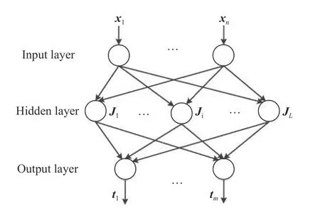
Fig. 1 Structure diagram of basic ELM

Given the training data setwith N samples,where xj∈Rnxis the input vector and tj∈Rnyis the corresponding expected output class label. Equation (1) can be written in a matrix form:

where the network hidden layer output matrix is

The output weight between the hidden layer and the output layer can be obtained by solving the least squares solutions of the following equations:

In (4), the first term is the regularization term against over-fitting, and the second is the error vector, and λ is the penalty coefficient. By setting the gradient of the ELM with respect to β to zero, we can get the following equation:

When the hidden matrix J is the full column rank,which means the number of training samples is larger than the number of hidden neurons, (5) can be solved as follows:

where ILis the identity matrix of dimension L, which is a square matrix where diagonal elements are “1” and others are “0”.

Otherwise, when the hidden matrix J is the full row rank, which means the number of the hidden neurons is larger than the number of training samples, the output weights of the ELM can be solved as follows:

where INis the id entity matrix of dimension N.

2.2 Constraint parameter setting method

Although setting input weights and bias based on experience can accelerate the learning speed of the ELM, it does not guarantee that all hidden layer nodes are useful.The generalization performance of the ELM is based on many hidden layer nodes. The larger the number of hidden layer nodes is set, the more time is spent in the training process, and it is more likely to over-fit. Therefore, in order to avoid such problems, we will introduce a new method to calculate weights from the input layer to the hidden layer and the hidden layer bias.

In [24], Su et al. proved that using difference vectors composed of different classes of sample data is effective for classification tasks. According to the conclusion, we randomly select the weight vector ai=[ai1, ai2, ···, ainx] of the ELM from the closed set composed of difference vectors of between-classes samples, instead of the parameters selected from the arbitrary open set. In fact, the essence of input weights is to map the original samples from one space to another feature space, which is convenient for sample classification. As shown in Fig. 2,where the rectangular represents the original space of the sample, the circle is the feature space, and the original sample represented by the triangle is mapped into the sample represented by the pentagram. When the weight vector from the input layer to the hidden layer is generated completely and randomly, the mapping result of one sample is shown in Fig. 3(a), which is not conducive to the classification of samples.

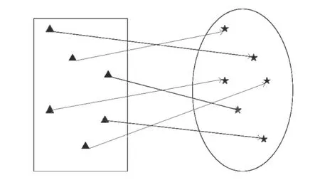
Fig. 2 Description of the sample mapping to the feature space

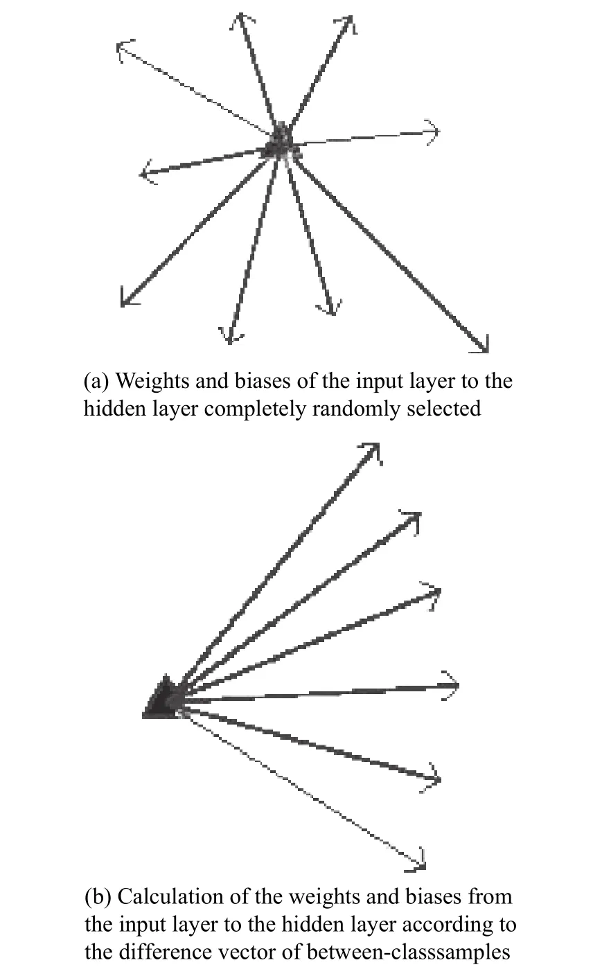
Fig. 3 Description of the influence of parameter selection on sample mapping results

We construct the parameters of the hidden layer according to the difference vector composed of between-class samples, so as to divide the sample into different regions in the feature space. For instance, xl1represents the sample data labeled l1, and the sample data labeled l2 is represented by xl2. After processing from the input layer to the hidden layer, xl1is mapped to the positive half axis of the feature space while xl2is mapped to the negative half axis. a is the weight from the input layer to the hidden layer, which can be expressed as λ(xl1−xl2), where λ is a normalized factor. Equation (8) can be converted to (9):

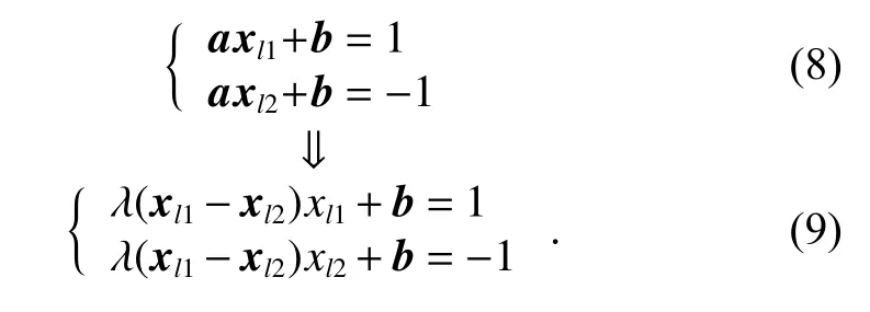
Normalization factor λ and bias b can be obtained by solving (9):

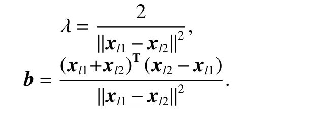
Therefore, the input weight can be expressed as

Fig. 3(b) shows the weights and biases of the input layer to the hidden layer calculated from the difference vector formed by the between-class samples, and it can be seen from Fig. 3 that this method makes the mapping of samples more regular.

2.3 Majority voting method

When the ELM is trained, the parameters are generated randomly and remain unchanged during the training process. Therefore, in the classification problem, some samples may be misclassified, especially when the sample data are closed to the classification boundary of the ELM construction [25]. For example, for a two-class problem,as shown in Fig. 4(a), the label of the triangle sample near the classification boundary should be red, and the result is misclassified as a green label in this ELM. Since the hidden layer parameters generated by each ELM are different, the classification boundary of the construction will be also different. In Fig. 4(b) and Fig. 4(c), the triangle samples near the classification boundary are correctly classified.

Through the above analysis, the classification result based on individual ELM may not be accurate. In order to reduce the mis-classification rate, multiple ELMs are combined and majority voting is utilized [26] to make decisions according to the idea of “the minority is subordinate to the majority”. In Fig. 4, after the classification results of the triangle sample near the classification boundary are counted in three different ELMs, the correct classification results can be obtained.

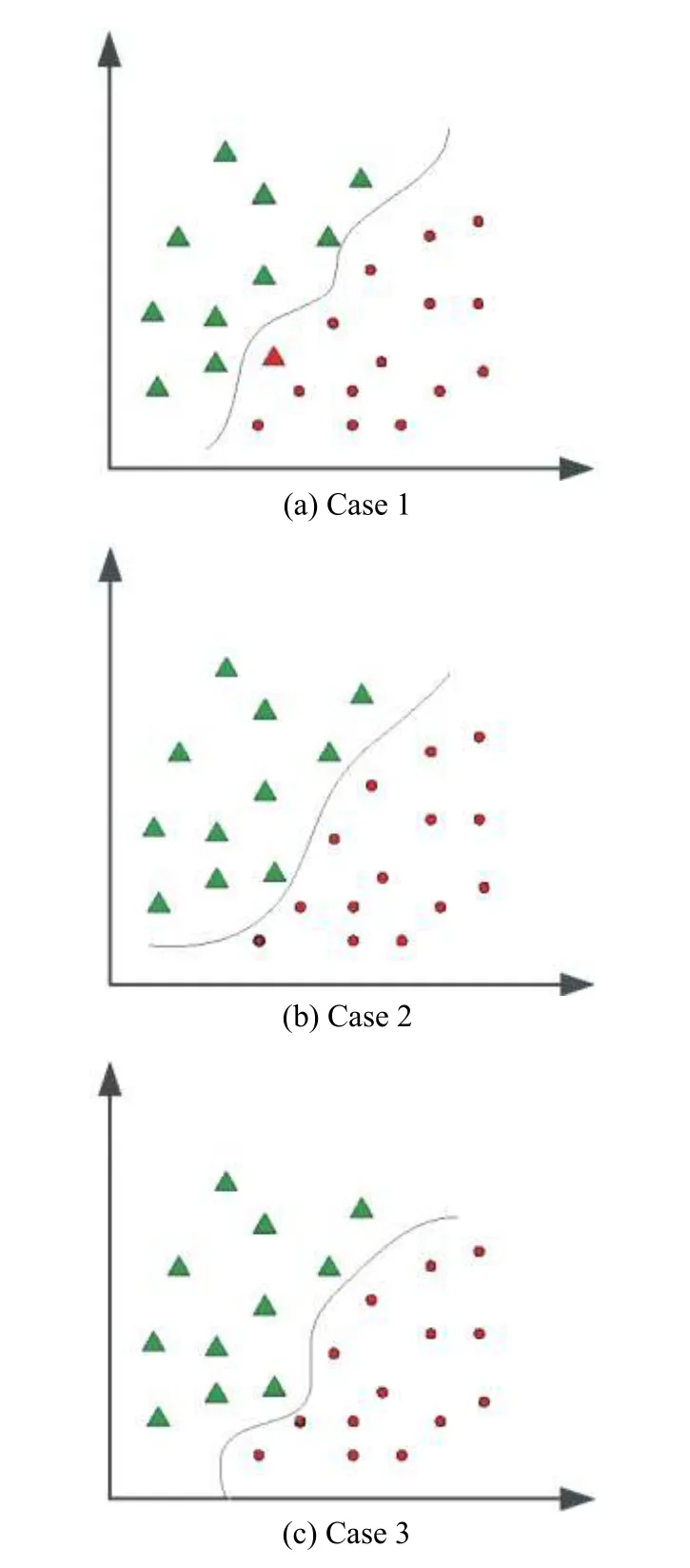
Fig. 4 Classifiers using ELM with different random parameters

In the majority voting algorithm, assuming that there are M weak learners, the corresponding vector VM,x(i)∈RCis used to store the output of each weak learner with the same dimension as the number of class labels, the initial element of which is zero, where i ∈[1,2,···,C]. When the class label predicted by the mth weak learner is class i,the element representing the class label i in the correlation vector V is incremented by one, such as

When all the class labels predicted by the weak learner are counted, the class label i represented by the largest value VM,x(i) is selected as the final prediction result:

The detail of the majority voting algorithm procedure is stated in Algorithm 1.

Algorithm 1Majority voting algorithm

InputThe dataset

Number of integrated weak learners: M.

The corresponding zero valued vector VM∈RC,VM,x(i)is the ith factor of VM, and C is the number of categories of samples.

OutputThe prediction classof the samplexj.

Step 1set m = 1

Step 2while ( m ＜M) do

Step 3The trained weak learning machine model is used to predict the class of sample x, and the result is stored in VM∈RC.

Step 4VM,x(i)=VM,x(i)+1

Step 5m=m+1

Step 6end while

Step 7The final prediction category of sample x is Cx=argwhere i ∈[1,2,···,C].

Step 8

ReturnSample xjfinally predicts class

3. The proposed framework

The detail of the CV-ELM algorithm procedure is stated in Algorithm 2.

Algorithm 2CV-ELM algorithm

InputTraining set

Activation function J(x).

Number of hidden layer nodes L.

Number of integrated ELMs:M.

OutputThe prediction classof the sample

Step 1setm=1

Step 2while ( m ＜M) do

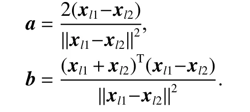
Step 3Randomly extract sample data xl1and xl2from two different categories of datasets to obtain a difference vector xl1−xl2.

Step 4Calculate the input weight a and bias b of ELM:

Step 5Calculate the hidden layer output matrix J as

Step 6Calculate the hidden layer’s output weight matrix β.

Step 7m=m+1

Step 8end while

Step 9The majority voting method is used to predict the result

ReturnThe predict classof the sample xj.

The proposed CV-ELM is illustrate in Fig. 5. In the training phase of the proposed CV-ELM algorithm, the difference vector composed of between-class samples is r andomly selected to calculate the input weigh a connecting the input layer to the hidden layer and the bias b of the hidden layer. M independent ELMs are trained to obtain the output weigh β and the parameters (a,b,β) of each ELM. In the test phase, the trained M based ELM models are used to predict the samples, and the experimental results are obtained. The final test result Cxis counted according to the majority voting method. Fig. 6 describes the procedure of the CV-ELM algorithm.

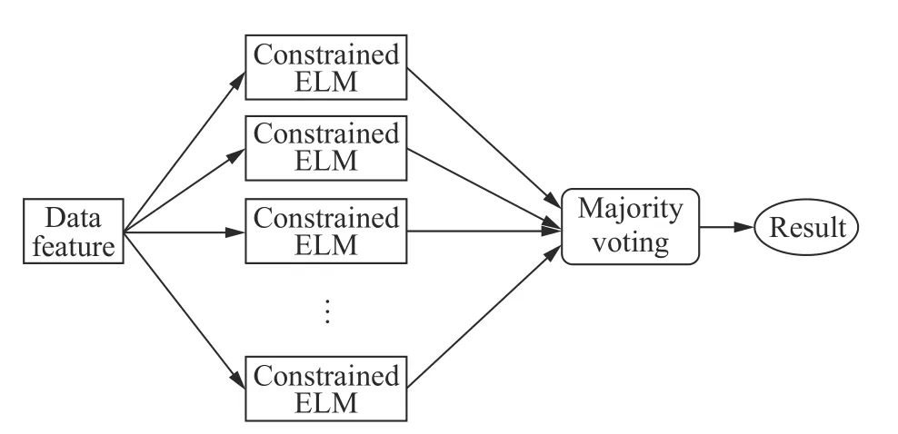
Fig. 5 Procedure of CV-ELM modeling algorithm

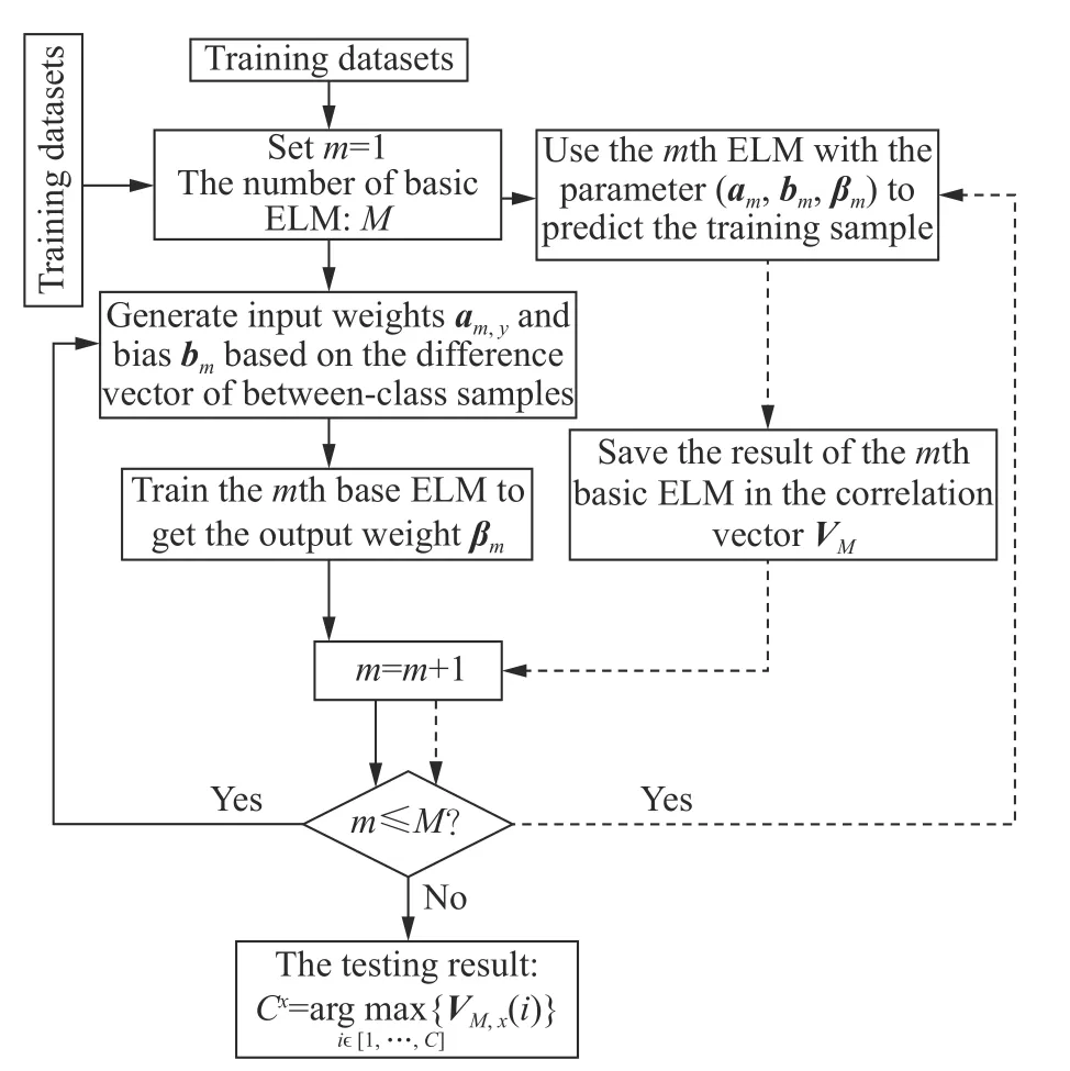
Fig. 6 Procedure of CV-ELM modeling algorithm

4. Experiment results

In this section, the proposed CV-ELM is compared with the original ELM [27], C-ELM (The hidden layer parameter of the ELM is calculated according to the betweenclass samples) [28] and V-ELM (ELM based on majority voting) [29], and the sigmoid activation function is used in all ELMs [30]. At the same time, the CV-ELM is also compared with some advanced classification methods.Furthermore, we use the proposed method to classify the SD state of the aluminum electrolysis industrial process and compare it with some state-of-the-art methods.

The experiment environment is based on Matlab R2014b running on a 2.5 GHz i7-6500U CPU with 12 GB RAM.

4.1 Experiment result on public datasets

In this subsection, we compare the performance of the CV-ELM with the original ELM, C-ELM and V-ELM by using eight public datasets. All experimental data are downloaded from the UCI database. Table 1 shows the details of the eight public data sets.

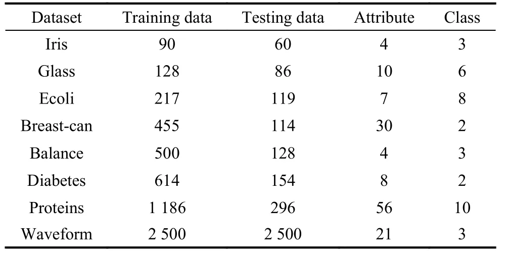
Table 1 Description of experimental data

(i) Comparison to the ELM: The number of hidden layer nodes in the ELM increases gradually from zero, and then the appropriate number of hidden layer nodes is selected based on the cross-validation method [31]. In both VELM and CV-ELM, 10 basic independent extreme learning machines are used. Table 2 gives the classification accuracy of eight public datasets. The training time and the number of the hidden layer nodes set in the CV-ELM are given in Table 3. It can be seen from the experimental results that the proposed CV-ELM is better than the ELM, C-ELM and V-ELM in classification accuracy.However, the training time of V-ELM and CV-ELM algorithms is longer than that of ELM and C-ELM. This is because the majority voting method is used in V-ELM and CV-ELM, so it takes time to train every basic ELM.Fig. 7 is the experimental results of the comparison between ELM and CV-ELM. It can be seen that the curve of CV-ELM’s test accuracy is always higher than that of ELM, and in all datasets, the use efficiency of hidden layer nodes in the CV-ELM is higher than that in the ELM.The experimental results show that setting the hidden layer parameters according to the difference vectors of the between-class samples can improve the use efficiency of the hidden layer nodes. The performance of the CV-ELM is better than the original ELM.

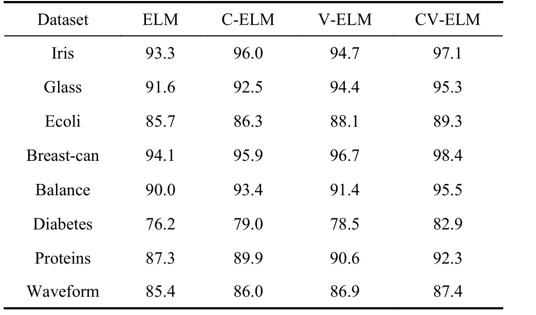
Table 2 Testing accuracy of experimental data %

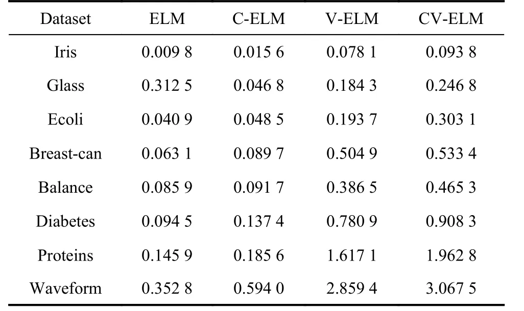
Table 3 Training time of experimental data s

(ii) Comparison to several advanced learning algorithms: Experiments are performed on eight previous public datasets using SVM [6], BP [32], deep long short term memory (LSTM) network [33], and the proposed algorithm. For the SVM, the activation function is the Gaussian radial basis function (RBF), and the penalty parameter C and the kernel parameter G are selected from C=[212,211,···,2−2] and G=[24,23,···,2−10], respectively [6]. For BP, the Levenberg-Marquardt algorithm is used to train the neural network. For deep LSTM network, two LSTM layers of sizes 20 and 35 are used. In the CV-ELM, the sigmoid activation function is used, and 10 independent ELMs are used for voting. Table 4 shows the detailed comparison results of the performance of CVELM and SVM, BP and deep LSTM methods, in which the highest test accuracy of each group of data is indicated in bold. As can be seen from Table 4, the CV-ELM algorithm has the highest test accuracy in the eight datasets, while in the Balance dataset, the accuracy rates of SVM and CV-ELM are similar. Deep LSTM has the highest accuracy in the Protein dataset, which is 1.2%higher than that in CV-ELM, but deep LSTM takes much longer training time than CV-ELM. From the perspective of training time, for all the public datasets, the learning speed of CV-ELM is much faster than SVM, BP and deep LSTM. According to the experimental results, the proposed CV-ELM algorithm has better performance.

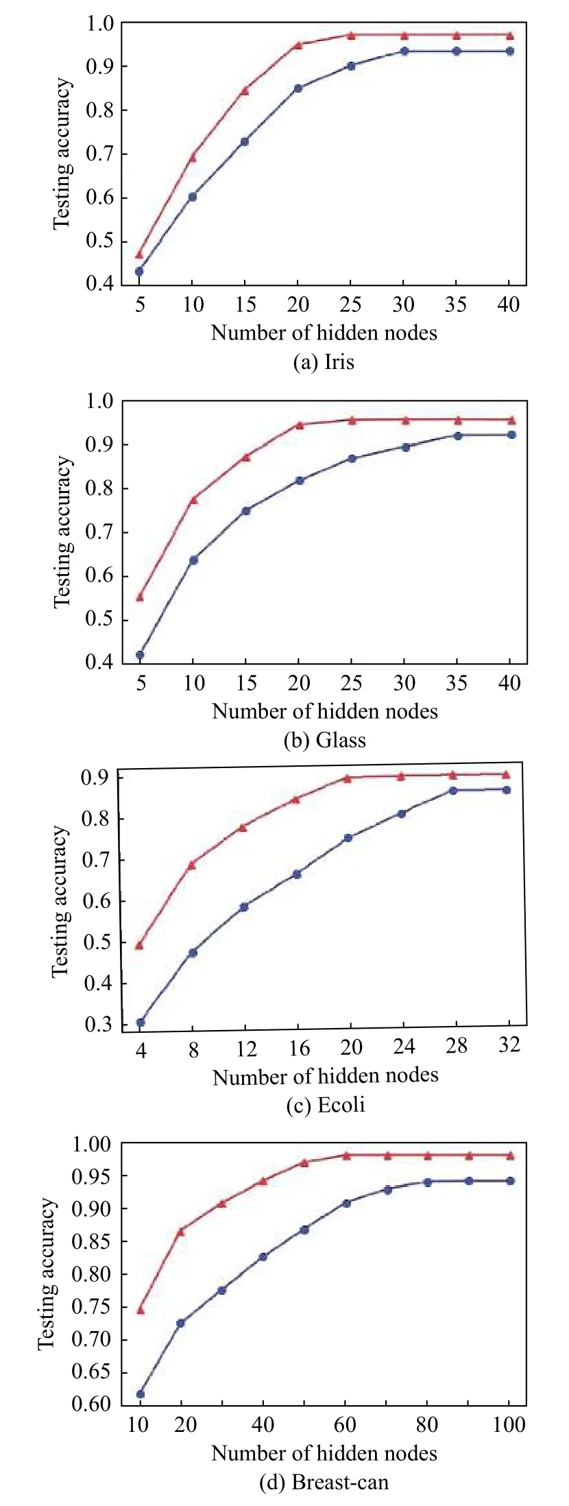
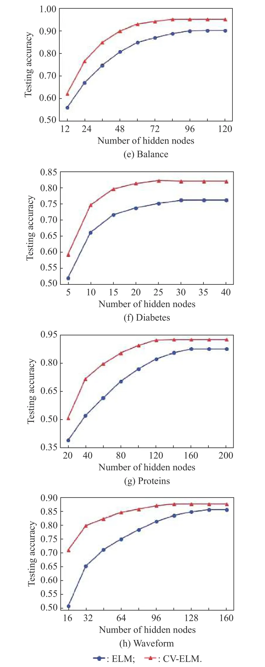
Fig. 7 Experimental results of the ELM, CV-ELM on public datasets

4.2 Application on SD classification in industrial aluminum electrolysis

In this subsection, the CV-ELM is used for SD identification of the aluminum electrolysis industrial process. SD is one of the important indexes to evaluate the production status of the electrolytic cell in aluminum electrolysis industry, which refers to the difference between the initial crystal temperature and the electrolyte temperature [34-36]. Usually, when the SD is between 2oC and 8oC, the electrolytic cell is considered as a “COLD” label. When the SD is between 8oC and 15oC, the electrolytic cell is considered as a “NORMAL” label, while the SD exceeds 15 °C, the electroytic cell is “HOT” label [37,38]. The traditional method of measuring SD is based on the operator’s decision, the method is time-consuming and cannot meet the requirements of modern aluminum electrolytic production. In the aluminum electrolytic production process, in order to improve the production efficiency and ensure the quality of aluminum, the production process must be detected in real time and judged in a timely manner [39]. The details of the electrolytic cell are shown in Fig. 8.

Table 4 Performances of CV-ELM and several advanced learning algorithms with the public datasets

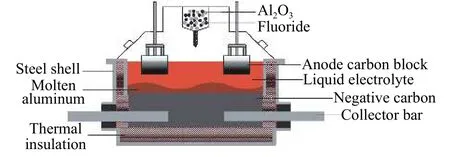
Fig. 8 Schematic diagram of the aluminum reduction cell

As the CV-ELM output is constant, the root mean squared error (RMSE) index is used to evaluate the performance of the algorithm, the calculation formula is given as

where yiis the actual label,is the value predicted by the model, and N is the number of the test samples.

Eight industrial process variables affecting the SD state are selected as input variables [40], and detailed information is given in Table 5. The normalized range of all data is[-1, 1]. In the experiment, 600 sets of data are used, of which 480 are randomly selected as training datasets and the remaining 120 are test datasets.

Fig. 9 is the classification accuracy of the CV-ELM with the number of the basic ELM from 10 to 100. We can see that when the number of basic ELMs is less than 40, the accuracy rate increases with the increase of the number of ELMs, while when the number of basic ELMs is greater than 40, the accuracy rate does not change much. Considering that the larger the basic ELMs are set,the longer training time it will take, it is appropriate to select 40 basic ELMs in the CV-ELM.

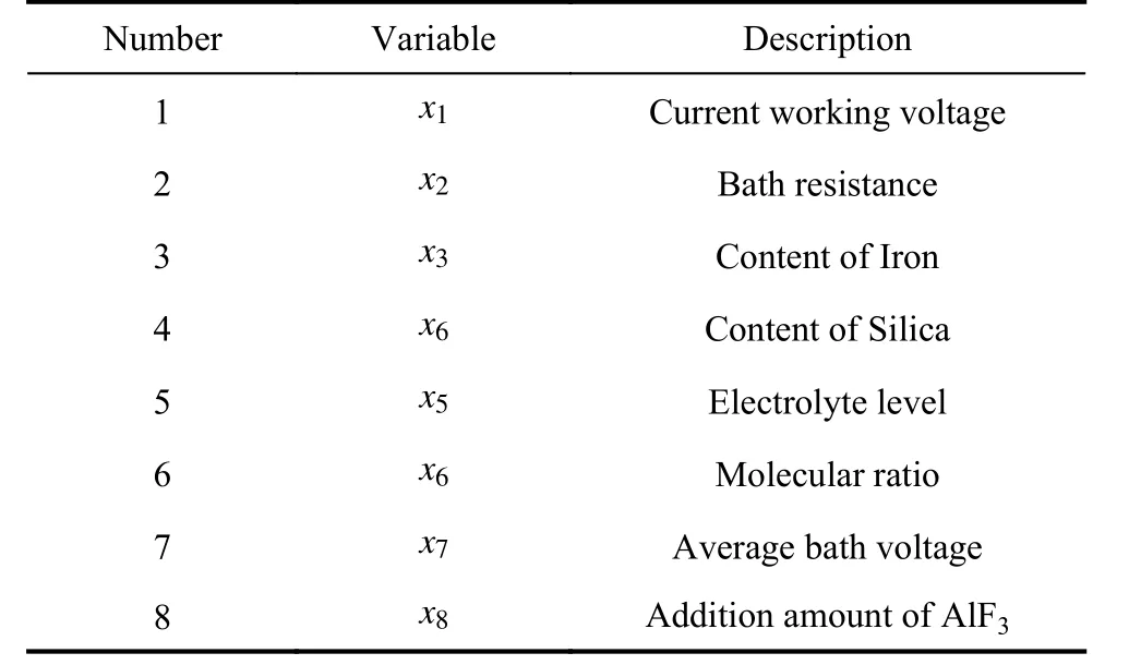
Table 5 Selected process variables according to operator experiences

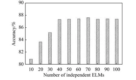
Fig. 9 Classification accuracies of the CV-ELM with the number of basic ELM from 10 to 100

Table 6 shows the experiment results in SD identification with different methods, such as deep belief network(DBN) [41], convolution neural network (CNN) [42],stacked autoencoder (SAE) [43], random forest (RF) [44],ELM [45], multilayer ELM (ML-ELM) [46]. For DBN,we set the epoch to 5, the batchsize to 20, the parameter momentum m is selected from [0.01,0.02,···,0.1], the learning rate α equals 1 −m. For SAE, the batchsize is set to 20, the learning rate α equals 1, and the parameter masked fraction rate is 0.5. For CNN, the Relu function is used as the activation function. The batchsize is set to 20,and learning rate α equals 0.005. One hundred decision trees are used in RF. For ML-ELM, the hidden layer is set to 2, the network architecture is 8-300-200-3. Among them, the CV-ELM has the highest classification accuracy, while the method based on artificial experience has the lowest accuracy. Compared with other methods, the CNN takes longer time in training time. Since it takes time to train each base ELM in the CV-ELM algorithm,the total training time spent on the CV-ELM is longer than that of the traditional ELM. However, in terms of identification accuracy, the CV-ELM is 6.8% better than the ELM. In the classification of the SD state in the process of aluminum electrolysis industry, the identification accuracy is very important within the allowable range of time. Considering the identification accuracy and training time, the performance of the CV-ELM is relatively better.

Table 6 Experiment results in SD identification with different methods

We compare the performance of the ELM and the CVELM. Fig. 10 shows the recognition accuracy of the CVELM and ELM methods with hidden nodes from 10 to 100. It can be found from Fig. 10 that the accuracy of the two algorithms will increase with the increasing hidden nodes, but they become stable when the number of hidden nodes is larger than a certain number. However, the more hidden nodes, the longer the training time. The CVELM has a good performance when the number of hidden layer nodes reaches 50, and the ELM requires 70 hidden layer nodes to achieve the same good performance.At this time, the accuracy of the CV-ELM test is 6.8%higher than that of the ELM, even if the CV-ELM has 20 fewer hidden layer nodes than the ELM. The test accuracy of the CV-ELM has always been higher than that of the ELM. The experiments show that the CV-ELM has a better generalization ability than the ELM.

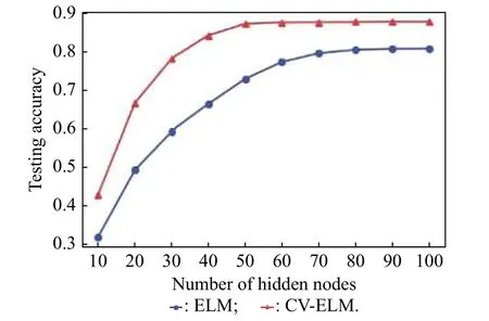
Fig. 10 Recognition accuracies of the basic ELM and the proposed CV-ELM with the number of hidden nodes from 10 to 100

5. Conclusions

In order to reduce the impact of random generation of hidden layer parameters on ELM learning performance,in this paper, we calculate the weight of connecting from the input layer to the hidden layer and the bias of the hidden layer by combining the difference vector of betweenclass samples. Meanwhile, a novel learning algorithm—CV-ELM is proposed by referring to the majority voting algorithm. The proposed method uses several public datasets to verify the performance and compares it with the traditional ELM and V-ELM. The experimental results show that the CV-ELM can not only improve the use efficiency of the hidden node in the ELM, but also could get a better accuracy rate. We also make a comparison with some state-of-the-art approaches for the SD states identification in aluminum electrolysis industry, the experiment results show that the CV-ELM classification accuracy rate reaches 87.4%, which has the good robustness and generalization ability. Further, the CV-ELM can be applied to solve other classification problems, and extended to more application areas.