A sparse algorithm for adaptive pruning least square support vector regression machine based on global representative point ranking

HU Lei, YI Guoxing, and HUANG Chao

School of Astronautics, Harbin Institute of Technology, Harbin 150001, China

Abstract: Least square support vector regression (LSSVR) is a method for function approximation, whose solutions are typically non-sparse, which limits its application especially in some occasions of fast prediction. In this paper, a sparse algorithm for adaptive pruning LSSVR algorithm based on global representative point ranking (GRPR-AP-LSSVR) is proposed. At first, the global representative point ranking (GRPR) algorithm is given,and relevant data analysis experiment is implemented which depicts the importance ranking of data points. Furthermore, the pruning strategy of removing two samples in the decremental learning procedure is designed to accelerate the training speed and ensure the sparsity. The removed data points are utilized to test the temporary learning model which ensures the regression accuracy. Finally, the proposed algorithm is verified on artificial datasets and UCI regression datasets, and experimental results indicate that, compared with several benchmark algorithms, the GRPR-AP-LSSVR algorithm has excellent sparsity and prediction speed without impairing the generalization performance.

Keywords: least square support vector regression (LSSVR),global representative point ranking (GRPR), initial training dataset, pruning strategy, sparsity, regression accuracy.

1. Introduction

The support vector machine (SVM) is a data learning method based on the structural risk minimization principle and Vapnik-Chervonenkis (VC) dimension theory [1].The time complexity of the SVM iswhich is hard to deal with large scale datasets, hence finding a novel SVM method with low computation cost is of great necessity. The least square support vector machine (LSSVM) utilizes the square loss function to replace the εinsensitive loss function in the SVM, transforms the quadratic programming problem in the SVM into the linear equations with the equality constraint, which greatly reduces the complexity of the calculation. The LSSVM has been successfully applied in a wide range of fields, such as forecasting [2-5], decision making [6], and target recognition [7]. However, the solutions of the LSSVM are not sparse, that is, the number of support vectors is equal to the number of training data, which makes the model complex and difficult to solve. Therefore, how to obtain the sparse solution of the LSSVM is the focus of many scholars [7-10].

Suykens [11] is the first author who proposed a sparse least square support vector regression (S-LSSVR) method.According to the support vector spectrum, the pruning strategy is designed, and the stop condition is that the prediction accuracy descends to the pre-designed accuracy threshold. Since then, many scholars [8,12-15] have proposed many methods to obtain the sparse solution of the LSSVM. Hong et al. [8] utilized the simplex basis function to get the sparse solution of S-LSSVR and verified the effectiveness of the proposed algorithm in several datasets. Yang et al. [12] utilized the orthogonal matching tracking algorithm to compress the training dataset so as to realize the sparsity of the LSSVM. Furthermore,Yang et al. [13] utilized the non-random matrix to replace the original random Gaussian matrix on the basis in [12].Experimental results showed the effectiveness of the proposed algorithm. In order to acquire the sparse solution of the LSSVM, De et al. [14] adopted the entropy-based core band width selection strategy and the fast cross validation method, and Karsmakers et al. [15] used the sparse conjugate direction pursuit sparse method to reduce the support vector set of the LSSVM. Cauwenberghs [16]proposed an LSSVM method based on incremental learning and decremental learning, and some scholars [17-19]put forward many innovative ideas and applications of the LSSVM based on incremental learning and decremental learning. Chen et al. [17] proposed the online incremental and decremental learning algorithm based on the variable SVM, and the experimental results showed that the algorithm given in the case ensured the correct classification rates and effective training’s speed. Lee et al. [18] gave a pre-trained model to adapt the changes in the training dataset, without retraining the model on all the data. Jin et al. [19] proposed a novel solution for incremental and decremental extreme learning machines based on recursively computing the left pseudo inverse of the hidden layer output matrix. The regression and classification experiments showed the feasibility and effectiveness of the proposed algorithm.

Zhao et al. [20] proposed two sparse LSSVR methods by defining a contribution function to the objective function based on recursive reduced LSSVR. The experiment results depict that the proposed methods [20] can get the sparsity to a certain degree. Jiao et al. [21] introduced a fast-greedy algorithm to the LSSVM (FGA-LSSVM),which is effective to overcome the non-sparseness of the LSSVM. On this foundation, a probabilistic speedup scheme was designed to improve the speed of FGA-LSSVM.Guo et al. [22] utilized the k-nearest neighbors to reduce the training data set which is effective to reduce the computational complexity. On this foundation, Zhao et al. [23]proposed an improved scheme which further reduced the computational complexity. Kruif et al. [24] proposed a pruning error minimization (PEM) in the LSSVM, that is,the sample with the minimal leave one error is pruned,which is effective to the sparsity of the LSSVM. Zeng et al. [25] introduced the sequential minimal optimization method into the pruning process and pruned the data point that will introduce the minimum changes to a dual objective function. Experiment results reveal the effectiveness of the proposed method in terms of computational cost and classification accuracy.

Wu [26] proposed an adaptive iterative LSSVR (AILSSVR) to deal with the prediction problem, starting training from any two samples. The strategy of “prediction-learning-verification” is adopted, the algorithm does not need to pre-setup the support vectors set and the solution has a good sparsity. Gao et al. [9] proposed an improved adaptive pruning LSSVR (IAP-LSSVR) algorithm,which improved the AI-LSSVR algorithm in two aspects.For one thing, the three kinds of pruning strategies are employed to remove the samples corresponding to the minimum value of the support vector spectrum. For another, the verification mechanism is to use the removed samples to verify the temporary learning model. Both the AI-LSSVR and the IAP-LSSVR methods have some shortcomings. Starting training from any two samples makes the training process not oriented, which makes the computation cost expensive. Ma et al. [27] proposed an SLSSVM based on global representative points (GRPLSSVM), which took local density and global dispersion into consideration. The method selects the global representative data points to form the support vector set firstly,and then uses the support vector set to solve the hyperplane of classification decision. According to the current research, the iterative algorithm based on incremental and decremental learning is still the main research direction[9,17-19], but there still exits some problems in practical applications, such as it is computed complexly because of the large size of the dataset, and its performance cannot meet the actual requirements, especially for the occasion with strong sparse requirements.

In this paper, we propose a novel adaptive pruning LSSVR algorithm based on global representative point ranking (GRPR-AP-LSSVR). The contribution of this paper is concluded as follows.

(i) A global representative point selection algorithm based on data density and dispersion is given in this paper. In this case, we build the initial sample working set,which allows that the incremental learning could start from the most significant samples.

(ii) In the decremental learning process, the pruning strategy adopted in this paper is to simultaneously remove two least important samples in the working set. The removed samples are utilized to verify the temporary learning model, which ensures the model accuracy.

(iii) Experiments conducted on artificial datasets and UCI regression datasets indicate that the proposed algorithm performs better in sparsity and prediction time compared to the benchmark pruning methods.

This paper is organized as follows. Section 2 introduces some fundamental theory knowledge. Section 3 presents the elaborate algorithm proposed in this paper. In Section 4, several experiments are conducted. Section 5 states the conclusions of this paper.

2. Related theory

2.1 LSSVR

Suppose that the training dataset in feature space is denoted asN is the size of the training dataset. xi∈Rdis sample i, d is the dimension of the input data, yi∈R is the output value, R represents the real number . The standard LSSVR can be formulated as the following quadratic programming (QP) optimization problem based on the equality constraints.

where ω is the weight vector, e is the error vector,γ∈R+is the regularization parameter which balances the model complexity and approximate accuracy. R+is the positive and real number. φ (·) is a nonlinear function which maps the input space into the high dimensional feature space,and b is a bias term.

The Lagrange function of the optimization problem is given as follows:

According to Karush-Kuhn-Tucker (KKT) conditions,the following formula is acquired.

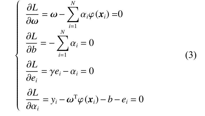
The linear system of equations can be deducted by eliminating the weight vector ω and error vector e.

Let V=Ω+γ−1I, named the kernel matrix, according to Mercer’s theorem, if the kernel matrix is invertible, the solution to (4) is acquired.

The regression function of the LSSVM is as follows:

Accor ding to γei−αi=0 from (3), the training erroreiis not equal to zero, consequently the parameteris not equal to zero,which means that all training samples become the support vectors, that is, the solutions are not sparse. In practical applications, the non-sparse solutions not only increase the storage burden but also prolong the prediction time. Consequently, it is indispensable to research the pruning method to get the sparse solutions.Consequently, the incremental learning and decremental learning [16] are introduced in the next section.

2.2 Incremental learning

Suppose that the LSSVR model of working set P including n samples has been built, and the kernel matrix can be denoted as

If a new data point (xn+1,yn+1) is added in the working set P, that is, P=P+{(xn+1,yn+1)}, the kernel matrix can be updated:

where

The computation cost of the inverse calculation of the updated kernel matrix Vn+1is intolerable with the increasing of the scale of the training set. In this case, a method for calculating the inverse kernel matrixbased onis introduced in this paper. There are two relevant lemmas.

Lemma 1Block matrix inversion

Lemma 2Matrix inversion

There are matrices A, B,C and D, A−1and C−1exist,then the following formula can be acquired:

According to Lemma 1 and Lemma 2, the inverse kernel matrixcan be denoted as follows [28]：

2.3 Decremental learning

Suppose that the LSSVR model of working set P including n samples has been built, and the inverse kernel matrix is denoted asIf a data point (xk,yk) is removed from the working set P, that is, P=P−{(xk,yk)}, the inverse kernel matrixcan be updated according to the inverse kernel matrixThe decremental learning is the reverse process of incremental learning.

where

Interested scholars can refer to [16,28] for specific deduction of incremental learning and decremental learning.

3. The proposed method

3.1 Global representative point rank algorithm

The S-LSSVR [11] algorithm prunes a bit of points in the|αi|spectrum corresponding to the minimal value, while the AI-LSSVR [26] and IAP-LSSVR [9] algorithms start training with any two sample points selected as the initial working sample set, which cause a problem that the training process spends much time because of scanning each sample. Therefore, this paper introduces the global representative point ranking (GRPR) algorithm aiming at accelerating the sparse solution of regression problems. The GRPR algorithm is a method to get the importance ranking of data points by calculating the density and dispersion of data points in feature space.

Suppose that a training dataset in the feature space is denoted asN is the size of training dataset. xi∈Rdis sample i, d is the dimension of the input data, yi∈R is the output value. The definition of the distance between sample i and sample j can be denoted as

where k is the kernel function.

The density of sample i in δ-neighborhood of density ρ in feature space is defined as follows:

where I (z) is the indicator function denoted as

According to (15), the density of sample i is the number of the samples in the δ-neighborhood, and the dispersion of sample i is defined as the minimum distance from sample i to other points whose density is greater than that of sample i. Consequently, we can get the specific definition of the dispersion of sample i.

Relevant research [18] indicates that global representative points can be selected according to the density and dispersion in ρ−ς coordinate axis, that is, the bigger the density and dispersion are, the better the global representativeness is. Considering that the dimension of ρ andς are different, it is of necessity to map ρ and ς into the fixed interval (a,b), in that case, we can get the new density and dispersion denoted asandFinally, we can get the global representative index of sample i:

where the bigger the global representative indexis,the better the global representativeness of sample i is. The GRPR algorithm can be depicted in Algorithm 1.

In order to describe the effectiveness of the GRPR algorithm, the exponential function is utilized to produce some samples with Gaussian noise which is drew in Fig. 1.

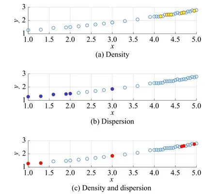
Fig. 1 Experimental result of GRPR algorithm

We adopt the density index, the dispersion index and the global representative index to analyze the data. Relevant experiment results are depicted in Fig. 1. In Fig. 1(a),the yellow solid circles represent the six sample points of the maximum density. In Fig. 1(b), the blue solid circles represent the six sample points of the maximum dispersion. In Fig. 1(c), the red solid circles represent the six sample points of the maximum global representative index. It is obvious that the representativeness of the red solid circles in Fig. 1(c) is excellent, which means that we can get the importance ranking of the dataset according to the GRPR algorithm.

Algorithm 1GRPR algorithm

InputS,k,δ

Output

Cacluate the matrix D.

Cacluate the density ρ and dispersion ς .

Cacluate the global representative index τ .

Sort the index τ in an asending order and sort the sample set.

3.2 GRPR-AP-LSSVR algorithm

Based on the GRPR algorithm, the ranked training dataset can be built, and pruning methods are designed to get the sparse solution to LSSVR. The pruning strategy of the AI-LSSVR [26] algorithm is to remove the point whose value of spectrum |αi| is the least. According to (3), we can get γei−αi=0, which denotes that the absolute value of training error is positively correlated with the absolute value of αi. Cawley et al. [29] gave the exact formula of leaving one error which denotes that the smaller the absolute value ofthe smaller the absolute value of training error, so the pruning strategy of the IAP-LSSVR[9] algorithm is to remove the point whose value ofspectrum is the least.

Both the AI-LSSVR algorithm and the IAP-LSSVR algorithm adopt a single pruning strategy, that is, there is at most one point which is removed in each decremental learning process, which limits the fast sparsity of the algorithm. Therefore, this paper adopts a pruning strategy that removes the two points corresponding to the minimal value of | αi|-spectrum andspectrum. The pruning strategy is divided into three cases to study. First, if the sample h and sample g represent the same sample,that is, h is equal to g, we can update the working setand then compute the updated inverse kernel matrixSecond, if the sample h and sample g represent the different samples and h is less than g, the working set can be updated asand then we can compute the updated inverse kernel matrixand then let h=h−1, compute the updated inverse kernel matrixand letThird, if the sample h and sample g represent the different samples and h is greater than g, we can update the working setcompute the updated inverse kernel matrixand then compute the updated inverse kernel matrixand letThe decremental learning based on pruning strategy (DLBPS) algorithm is described in Algorithm 2.

Algorithm 2DLBPS algorithm

Input

Output

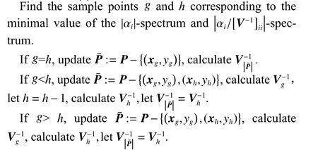
In order to reduce the model error brought by removing two points in each decremental learning process, we adopt a strategy of using the removed points to verify the temporary learning model, the specific process is depicted in Fig. 2.

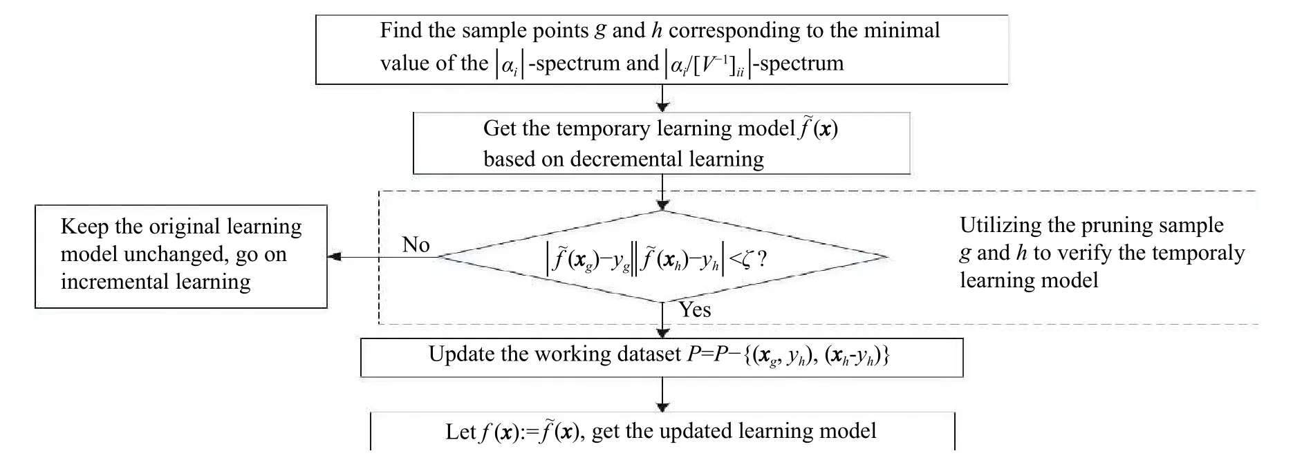
Fig. 2 Verification strategy of the temporary learning model

To be specific, we can find the sample points g and h corresponding to the minimal value of the |αi|-spectrum andspectrum, and compute the temporary learning model according to the DLBPS algorithm. Then we can compute the productifwhich indicates that the removed samples satisfy with the accuracy requirement, otherwise, keep the original learning model and go on incremental learning.

According to the above, we can get the pseudo code of the GRPR-AP-LSSVR algorithm which is depicted in Algorithm 3. In Step 1, compute the sorted datasetaccording to Algorithm 1. Build the initial wording dataset in Step 2. The kernel matrix and regression parameters can be computed in Step 3. In Step 4, we will scan each sample according the sequence of datasetwhere the more important the sample is, the earlier it is scanned,and Algorithm 2 and the verification strategy are utilized to judge whether the sample is a support vector. If all samples are scanned, then exit the loop. In Step 5, we can get the regression mode. It is worth noting that there is no need for repeated training of dataset because the working set in each step is certain, which is helpful to save the training time. This is the reason why we adopt the GRPR algorithm to rank the dataset before the training.

Algorithm 3GRPR-AP-LSSVR algorithm

InputS,ξ,δ,k

Outputα,b

Step 1Get the sorted datasetaccording to Algorithm 1.

Step 2Build the initial working dataset

Step 3Calculate the inverse kernel matrixand the regression parameters α|P|and b|P|.

Step 4Loop:L = 3:N

(i) If | f(xL)−yL|＜ξ, go to Step 4, otherwise, go to the next.

(ii) Expand the working dataset P=P+{(xL,yL)}.

(iii) Calculate the inverse kernel matrixand the regression parameters α|P|and b|P|according to the incremental learning.

(iv) Get the inverse kernel matrixand update working datasetaccording to Algorithm 2.

(v) Calculate the regressiong parameters

Step 5Get the parameters of the regression model,α:=α|P|, b:=b|P|.

3.3 Complexity analysis

Let N denote the training dataset size, solving the standard LSSVR problem is to solve the inverse kernel matrix, so the time complexity of the standard LSSVR algorithm can be depicted asLet ε denote the pruning ratio of the S-LSSVR algorithm, the time complexity of the S-LSSVR algorithm can be depicted asAccording to [9,26], let M denote the iteration number of AP-LSSVR and IAP-LSSVR algorithms, the time complexity of the AP-LSSVR and IAP-LSSVR algorithms can be depicted asThe incremental learning process of the GRPR-AP-LSSVR algorithm proposed in this paper is certain rather than random, so there is no need for repeated training of the dataset. The computational cost of the GRPR-AP-LSSVR algorithm includes two parts, the GRPR algorithm C1and the regression learning algorithm C2. The computational complexity of the sample ranking algorithm isthe computational complexity of the regression learning algorithm isTherefore, the computational complexity of the GRPRAP-LSSVR algorithm can be computed as C=C1+C2=consequently, the time complexity of the GRPR-AP-LSSVR algorithm is

4. Experimental results and analysis

4.1 Experiment design

Artificial datasets and UCI regression datasets are selected to verify the performance of the proposed algorithm in this paper. These selected datasets are of practical significance, specific details are described in Table 1.

Table 1 Description of datasets

As we know, the size of the support vector set depends on the learning accuracy parameter ξ, the smaller the learning accuracy parameter is, the bigger the size of the support vector set, the better the generalization performance of the model. We set ξ=0.01 in this paper. The regularization parameter γ and the kernel parameters of the radial basis function σ are selected respectively fromaccording to the cross validation method [29,30]. Detailed parameters setting is depicted in Table 2.

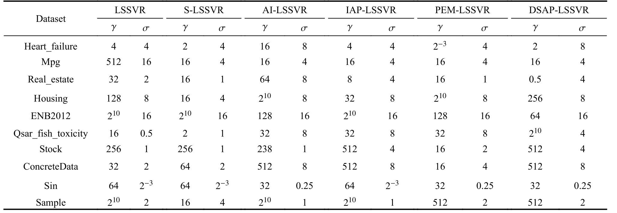
Table 2 Parameters setting

In the experiment, we compare the proposed algorithm with the standard LSSVR, S-LSSVR [11], AI-LSSVR[26], IAP-LSSVR [9] and PEM-LSSVR [24] algorithms.Five indexes, including support vector number (#SV),root mean square error (RMSE) of the test sets, Willmott’s index of agreement (WIA) [31], training time and test time, are selected to analyze the performance of the proposed algorithms. WIA is used to measure the regression degree, and the larger the WIA is, the more accurate the predicted results are. Furthermore, to make the results more credible, the ten-fold cross validation method is adopted to get the statistical average value. The RMSE index and the WIA index can be computed according to (19) and (20).

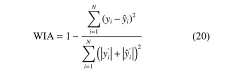
where yiis the real value,is the predicted value, and

4.2 Results and analysis

The experimental results are described in Tables 3-12.The regression graph of Sin and Sample datasets are depicted in Fig. 3 and Fig. 4, where the solid line is fitted by the training data, and the support vector is marked with“o”. The detail analysis is given as follows.

Table 3 Experimental result of Heart_failure dataset

First, the analysis of sparsity is given as follows according to Tables 3-12. The non-sparse solutions based on the standard LSSVR algorithm are given which can be regarded as a benchmark. The sparse solutions in UCI and artificial datasets are acquired based on the other five algorithms. It is obvious that the sparsity of the AI-LSSVR algorithm, the IAP-LSSVR algorithm and the PEMLSSVR algorithm is better than that of S-LSSVR, while the sparsity of the GRPR-AP-LSSVR algorithm proposed in this paper is the best. Furthermore, from Fig. 3 and Fig. 4, it is easy to observe that the sparsity of the GRPRAP-LSSVR algorithm in Sin and Sample datasets is the best over the other algorithms, which shows that the effectiveness of the pruning strategy designed in this paper can reach an excellent result when a strong sparsity is required. Although the RMSE of the GRPR-AP-LSSVR algorithm is not the smallest, it is accepted within a certain range. Especially in some practical application which requires strong sparsity, the proposed algorithm is valuable and reliable. The reason is that the GRPR algorithm is adopted to rank the dataset which allows the incremental learning process to start from a fixed direction.

Table 4 Experimental result of Mpg dataset

Table 5 Experimental result of Real_estate dataset

Table 6 Experimental result of Housing dataset

Table 7 Experimental result of ENB2012 dataset

Table 8 Experimental result of Qsar_fish_toxicity dataset

Table 9 Experimental result of Stock dataset

Table 10 Experimental result of ConcreteData dataset

Table 11 Experimental result of Sin dataset

Table 12 Experimental result of Sample dataset

Second, utilizing the RMSE index is of necessity to evaluate the regression accuracy of algorithms. Besides Sin and Sample datasets, the regression accuracy of several algorithms is in the same order of magnitude. In general, the regression accuracy of the standard LSSVR algorithm and the S-LSSVR algorithm are better than AILSSVR, IAP-LSSVR, PEM-LSSVR and GRPR-AP-LSSVR algorithms. In Sin and Sample datasets, the regression accuracy of the standard LSSVR method is the best,while the regression accuracy of AI-LSSVR, IAP-LSSVR, PEM-LSSVR and GRPR-AP-LSSVR algorithms are better than that of the S-LSSVR algorithm. In general, the regression accuracy of S-LSSVR, AI-LSSVR, IAP-LSSVR, PEM-LSSVR and GRPR-AP-LSSVR algorithms are obviously less than or equal to that of the standard LSSVR methods, and the regression accuracy of AI-LSSVR,IAP-LSSVR, PEM-LSSVR and GRPR-AP-LSSVR algorithms are basically in the same order of magnitude.Meanwhile, we can get the same results according to the WIA index which means that the GRPR-AP-LSSVR algorithm can achieve strong sparsity under certain accuracy requirements.

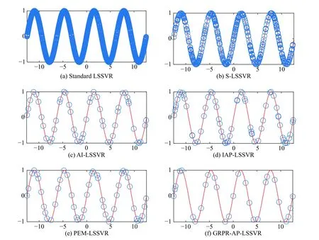
Fig. 3 Sin function regression

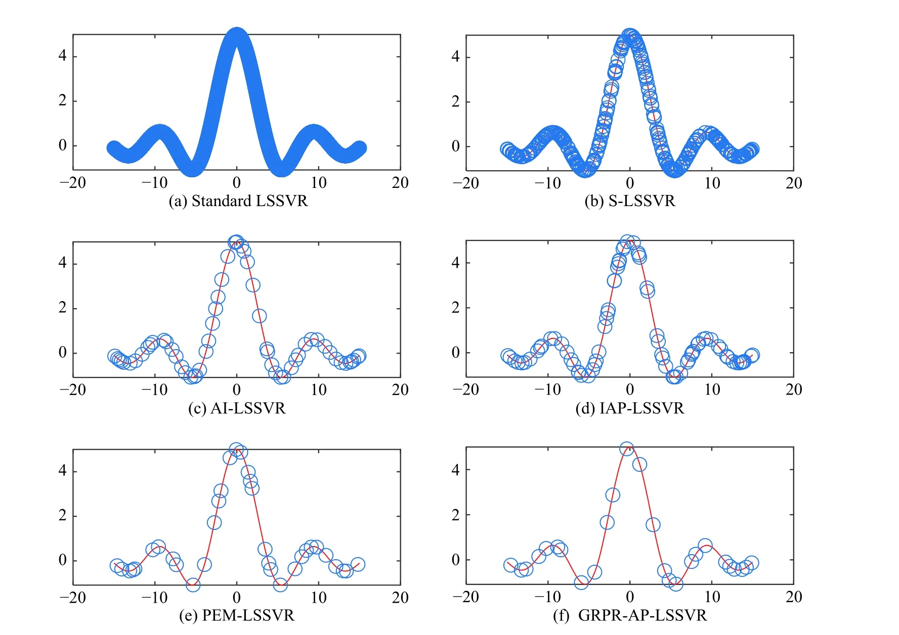
Fig. 4 Sample function regression

Finally, in terms of time consumption, the training time and testing time indexes are utilized to evaluate the rapidity of the algorithm. From Table 3 to Table 12, the training time of LSSVR and S-LSSVR algorithms increases with the increasing of the dataset size, while the training time of AI-LSSVR, IAP-LSSVR, PEM-LSSVR and GRPR-AP-LSSVR algorithms is not only affected by the dataset size, but by the number of the support vectors.According to Tables 7, 9, 11 and 12, the training time index of the proposed algorithm is better than the other algorithm, however, in Tables 3, 4, 5, 6, 8 and 10, we can summarize that the training time index of the GRPR-APLSSVR algorithm is better than AI-LSSVR, IAP-LSSVR and PEM-LSSVR algorithms, which presents the law that the larger the number of the support vectors is, the more time the training costs. From the aspect of testing time,the GRPR-AP-LSSVR algorithm has strongest sparsity,which has absolute advantage over the other algorithms.As a conclusion, the GRPR-AP-LSSVR algorithm has a strong rapidity in terms of training time and testing time.In this case, the GRPR-AP-LSSVR algorithm is extremely suitable for the fast prediction problem.

5. Conclusions

In this paper, aiming at the sparse problem of the standard LSSVR, a GRPR-AP-LSSVR method is designed.The proposed algorithm is helpful to eliminate the blindness of the scanning samples in the incremental learning process by sorting the training dataset through the GRPR algorithm, which can reduce the time consumption in incremental and decremental learnings. Furthermore, strong sparsity is got by the designed pruning strategy, which allows the proposed algorithm to deal with the fast prediction problem. As a conclusion, the algorithm proposed in this paper has the characteristics of strong sparsity and stable performance, which provides a new way to study LSSVR sparsity. Other data feature description methods will be taken into consideration for the future study.