NSHV trajectory prediction algorithm based on aerodynamic acceleration EMD decomposition

LI Fan, XIONG Jiajun, LAN Xuhui, BI Hongkui, and CHEN Xin

1. Air Force Early Warning Academy, Wuhan 430019, China;2. Unit 95980 of the PLA, Xiangyang 441000, China

Abstract: Aiming at the problem of gliding near space hypersonic vehicle (NSHV) trajectory prediction, a trajectory prediction method based on aerodynamic acceleration empirical mode decomposition (EMD) is proposed. The method analyzes the motion characteristics of the skipping gliding NSHV and verifies that the aerodynamic acceleration of the target has a relatively stable rule. On this basis, EMD is used to extract the trend of aerodynamic acceleration into multiple sub-items, and aggregate sub-items with similar attributes. Then, a prior basis function is set according to the aerodynamic acceleration stability rule, and the aggregated data are fitted by the basis function to predict its future state. After that, the prediction data of the aerodynamic acceleration are used to drive the system to predict the target trajectory. Finally, experiments verify the effectiveness of the method. In addition, the distribution of prediction errors in space is discussed, and the reasons are analyzed.

Keywords: hypersonic vehicle, trajectory prediction, empirical mode decomposition (EMD), aerodynamic acceleration.

1. Introduction

The trajectory prediction is only possible if the target maintains a certain regularity for a period of time after the prediction point. Generally speaking, the existing research on the prediction of aerial target trajectories can be roughly divided into two categories. The first one is the low-altitude flight path prediction for aircraft, unmanned aerial vehicle (UAV) and other targets. This type of target has strong maneuverability and complex movement modes. Fortunately, such target flight experiments and missions are frequent, and there are some routes and headings in a large amount of flight data. Therefore, the research hotspot of the trajectory prediction for this kind of target is how to mine the target intention and analyze the flight rules based on a large amount of flight data.The second category is the missile trajectory prediction.This type of target has a fast flight speed, which limits its maneuverability to some extent. Especially for ballistic missiles, its movement law is relatively stable after the engine is turned off (uniform motion). The research on the trajectory prediction of such targets focuses on how to analyze the rules of movement and then predict their trajectories. For the near space hypersonic vehicle (NSHV)trajectory prediction, on the one hand, there are fewer flight experiments and severely insufficient flight data; on the other hand, NSHV has a faster flight speed and its movement characteristics are closer to missiles, their movements have certain rules. The most existing NSHV trajectory prediction methods are based on missile trajectory prediction methods. However, compared to the ballistic target, NSHV has the ability to switch control modes and uses non-inertial ballistic flight. These factors make NSHV target trajectory prediction more difficult.

As we all know, equilibrium gliding and skipping gliding are two typical modes of flight for NSHV. Among them, the equilibrium gliding mode generally meets the zero-bank angle balance glide constraints [1,2], and its control instruction is greatly limited. In this flight mode,the NSHV maneuver mode is relatively single, and its trajectory prediction is relatively simple. When the NSHV is in the skipping gliding fight mode, it has greater freedom of control instructions. The target jumps vertically and may be accompanied by the lateral movement. Actually,the trajectory prediction for this flight mode is very difficult [3,4].

At present, most research works on the NSHV trajectory prediction mainly concentrate on the skipping gliding flight mode. Wang et al. [5] proposed a trajectory prediction method based on the lift-to-drag ratio. The method considers that the NSHV lift-to-drag ratio is linear, and the trajectory prediction is realized by fitting the lift-todrag ratio curve. However, it is only applicable to the longitudinal plane and cannot realize the 3D trajectory prediction. Zhang et al. [6] assumed that the prior information such as the equivalent area and mass of the target was known, and then identified the control amount to achieve the trajectory prediction based on the filtering result. The trajectory prediction effect is better when the target uses the typical control mode, but the assumption of prior information is too ideal (in fact, some prior information is basically impossible to obtain), which greatly limits the applicability of the algorithm. Yang et al. [7] used the strong nonlinear ability of the generalized regression neural network (GRNN) to fit the position to obtain the target’s future state. This method has good adaptability to different types of maneuvers, but it does not consider the target’s motion characteristics, resulting in unstable prediction errors. Li [8] proposed a trajectory prediction method based on the best maneuvering mode. This method considers that the acceleration of NSHV in the height direction is a form of attenuation oscillation, and the acceleration in the latitude/longitude direction is a combination of uniform acceleration, linear acceleration, and quadratic curve acceleration. It is reasonable for the acceleration assumption in the height direction, but it also shows that the acceleration rule in the latitude/longitude direction needs to be further analyzed.

In this paper, we propose a trajectory prediction method based on aerodynamic acceleration empirical mode decomposition (EMD). First, the aerodynamic acceleration distribution in the skipping gliding flight mode is analyzed,and it is verified that the aerodynamic acceleration has a stable rule. Second, the EMD is used to decompose the aerodynamic acceleration and extract trend terms. Third,in order to obtain the predicted data of aerodynamic acceleration, a prior basis function is set according to the law of aerodynamic acceleration and the corresponding parameters are obtained through data fitting. Finally, the trajectory prediction is achieved by using the aerodynamic acceleration prediction data to drive the motion differential equations to obtain the target state.

2. Aerodynamic acceleration characteristics

2.1 Target motion model

The motion differential equation of the NSHV can be simplified to (1) without considering the Earth’s rotation[9].

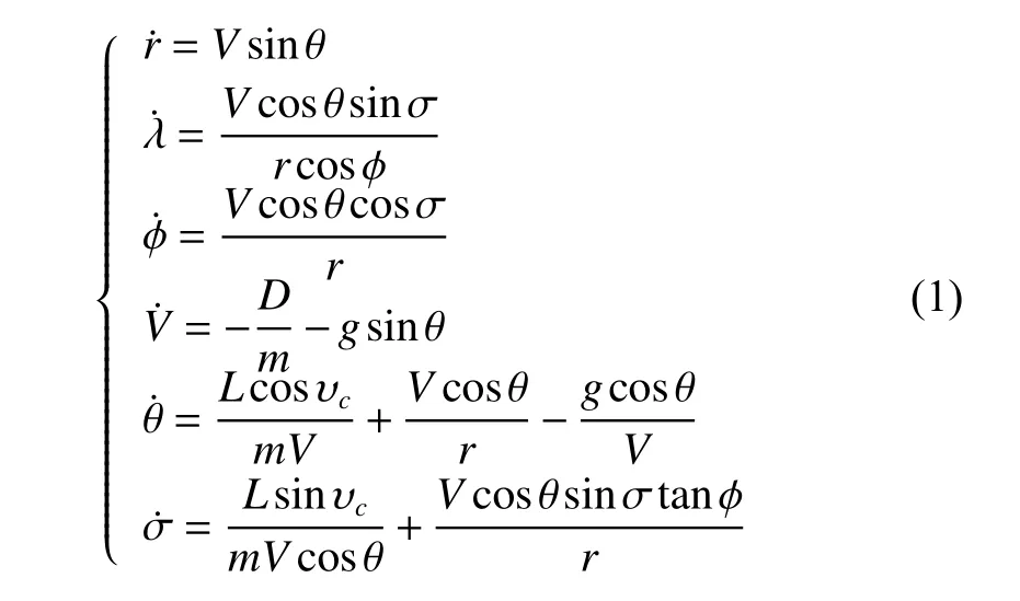
where m denotes the target mass, vcrepresents the target angle of bank, and g represents the gravitational acceleration.

On the basis of (1), r is the target geocentric distance,λis the target longitude, ϕ is the target latitude, V is the target velocity, θ is the target velocity dip, σ is the target velocity azimuth, L represents the lift and D represents the drag. The expressions of lift and drag forces can be simplified to

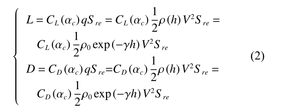
where m and Srerepresent the target mass and equivalent area respectively, CL(·) and CD(·) are the lift coefficient and drag coefficient respectively, q is the dynamic pressure, acis the target angle of attack, ρ(h) is the target local atmospheric density, ρ0is the standard atmospheric density, γ is the height constant, and h is the target height.

According to CAV-H public information, the lift and drag coefficient expressions can be found in [10].

2.2 Trend of aerodynamic acceleration

As we all know, for the skipping gliding flight mode, the NSHV is only affected by air lift L, air drag D and gravity G [11], where drag D is opposite to velocity V, and L⊥D , that is, the lift L only changes the direction of the speed but not the value. Therefore, the change in the speed value is only related to the air drag D and gravity G. The force of the target in the rising and falling stages is shown in Fig. 1. aL, aD, g represent the lift acceleration, drag acceleration and gravitational acceleration, respectively.

As shown in Fig. 1, during the trajectory rising phase,the gravity acceleration components gD=gsinθ and aDare opposite to the velocity direction. Thus, the speed is reduced.

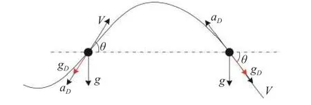
Fig. 1 Force analysis in the rising and falling stages

In the trajectory falling phase, aDis always opposite to the speed direction, but gDis consistent with it. At this time, the change of V depends on the sizes of aDand gD.According to [12-14], it can be known that gDis smaller because θ is smaller. Therefore, aDis the main factor affecting the change of V. To illustrate this in detail, we analyze the distribution of aDand gDthrough numerical simulation. (αc=15°, vc=0°, θ=6°and other parameters are shown in Table 1).

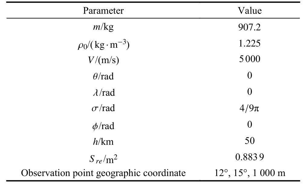
Table 1 Aircraft trajectory and observation sensor parameter

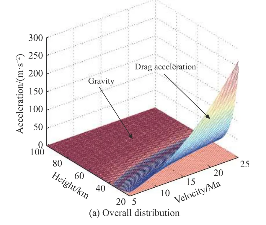
The distribution of aDand gDwith respect to velocity and height is shown in Fig. 2.

As shown in Fig. 2, for gD, its overall distribution is relatively stable, and it is not sensitive to changes in height and speed.

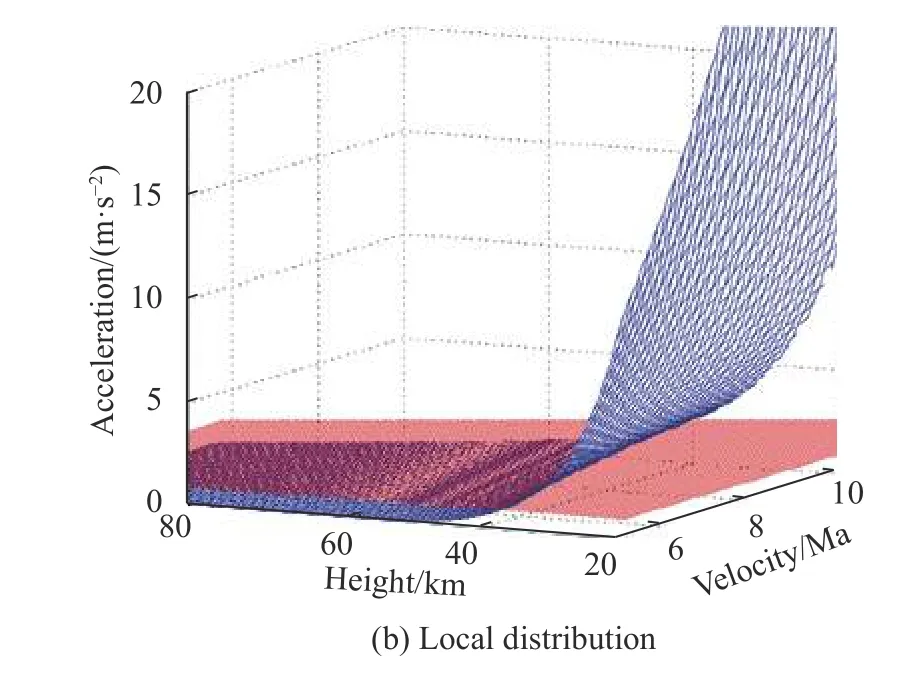
Fig. 2 Distribution of aD and gD with respect to velocity and height

The distribution surface of aDis mainly divided into two parts. In the first part, the height is about 40 km or more. In this part, the overall distribution of aDis stable,and its value is less than that of gD. In the second part, the height is below 40 km. At this part, the sensitivity of aDto height and speed is high, and its overall surface is above that of gD. Furthermore, the value of aDincreases rapidly as the height decreases or the speed increases. On this basis, we can analyze the change rule of aerodynamic acceleration according to aDand gDnumerical distribution.

Take lift acceleration aLas an example, as shown in Fig. 3, where the black curve is the target flight altitude and the red curve represents the lift acceleration. When the target reaches the peak height hBfrom hA, aLdecreases to the valley point due to the reduction of the target speed and air density. In the process from hBto the valley height hC, the speed decreases and the air density increases sharply. However, the speed base is large and aLis more sensitive to changes in altitude compared to speed. Therefore, aLpeak appears at hC, and then proceeds to the next hA, hBand hC.

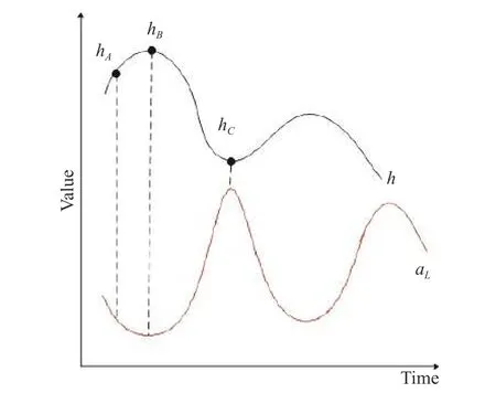
Fig. 3 Lift acceleration variation rule

In addition, we know that the expression for air density is

The rate of change of air density with respect to height can be obtained based on

It is noted that there is a negative correlation between the flying height and the rate of change of air density.That is, the lower the height, the faster the air density changes. This is the reason why the curve changes rapidly around hC, but is gentler near hBin Fig. 3. On this basis, taking into account the continuous changes in the target speed and air density, aLgenerally exhibits a resonance rule, and the oscillation amplitude decreases with time.

In the same way, it can be analyzed that the change rule of drag acceleration aDand lift acceleration aLis similar, but the amplitude is different.

3. Aerodynamic acceleration decomposition based on EMD

In Section 2, we verify that the aerodynamic acceleration of the skipping gliding NSHV has a stable resonance rule,which creates convenient conditions for the trajectory prediction. On this basis, we can set a prior basis function to predict aerodynamic acceleration, and then extrapolate the target state to achieve the trajectory prediction.However, it is difficult to characterize the resonance rule of aerodynamic acceleration. To solve this problem, first,the EMD is used to decompose the aerodynamic acceleration filtering results [15]. Second, the partially decomposed sub-items are selected for clustering. Thereafter, the clustered data are fitted and predicted by a prior basis function. Finally, the trajectory prediction is achieved.

As we all know, the NSHV trajectory prediction is a typical time-frequency data analysis problem. While traditional time-frequency analysis methods such as Fourier transform (FT), Hilbert transform (HT), and wavelet transform (WT) [16-18] are designed to extract or separate specific signal components from the data. These methods are based on powerful mathematical theories,and the extracted signal components are “standard”. Unfortunately, the resonance law of NSHV aerodynamic acceleration is not a strict mathematical expression, nor does it necessarily meet linear and stationary conditions.The traditional time-frequency analysis methods have some limitations in analyzing such data. To solve this problem, we use EMD to decompose the results of aerodynamic acceleration filtering [19-21]. The EMD is theoretically applicable to any type of data decomposition,and has very significant advantages in processing nonlinear and non-stationary data. In this paper, we decompose the data into simple sub-items through EMD, then merge similar items according to their time-frequency characteristics, and finally predict each similar item.

3.1 EMD algorithm

Assume that the time series of the drag acceleration isThe EMD decomposition of S(t) can be performed as follows.

3.1.1 Envelope and envelope mean

(i) Calculate all local extreme points of aD(t), and perform cubic spline interpolation on the local maximum and local minimum, respectively. Then get the corresponding upper and lower envelopes Lup(t) and Llow(t).

(ii) Calculate the mean of Lup(t) and Llow(t):

then there is

3.1.2 Intrinsic mode function (IMF)

The EMD-decomposed sub-items include IMFs and residual. In most cases, h1(t) still has obvious asymmetric differences after the envelope mean cancellation, and it cannot be directly used as the IMF. Therefore, we need to perform Step 1 and Step 2 with h1(t) as the original data,and continue to cancel its mean. Assume that the average envelope of h1(t) is m11(t).

The above process is repeated until the decision condition is satisfied between h1(k−1)(t) and h1k(t). While the first IMF i mf1(t) is

Considering the stability and physical significance of the IMF, Rilling et al. [22-24] proposed the mode amplitude (MA) and evaluation function (EF) decision criteria based on Huang[19].

MA(t) and EF(t) can not only ensure the stability of the IMF as a whole, but also allow local fluctuations. A sub-item must meet the two conditions to be considered an IMF. First, the proportion of data points satisfying MA(t)＜κ1is greater than 1−κ. Second, the data ratio that satisfies EF(t)＜κ2is at least κ. Furthermore, Rilling gave the reference values as κ=0.05, κ1=0.05, κ2=10κ1.

3.1.3 Residuals

After getting first IMF imf1(t), the remaining amount r1(t)can be expressed as

where r1(t) is the new data source.

Repeat Sections 3.1.1-3.1.3 to get multiple IMFs. The EMD decomposition is completed when the number of extreme points of rn(t) is less than 2. The following relationships exist in this process:

where rn(t) is the residual of the EMD. We can achieve the reconstruction of the original data through IMF vectorand residuals rn(t).

3.2 Sub-item selection and clustering

Essentially, the EMD is a screening process that extracts data with similar vibration patterns. There are multiple IMFs in the EMD decomposition of aerodynamic acceleration, and the selection and clustering of IMFs will directly affect subsequent predictions.

3.2.1 Sub-item selection

Generally, in the EMD decomposition sub-items, most of the high-frequency sub-items are filtering errors, with high frequencies and low energy. While low-frequency IMF and residuals represent trends and laws, with low frequencies and high energy. Therefore, only the low frequency sub-items are selected in the prediction process.In this way, we arrange the IMF and residuals in the ascending order of energy. With 95% of the total energy as the boundary, we select the top ranked item for the next clustering.

3.2.2 Sub-item clustering

The reasons for clustering sub-items are as follows:

(i) The fusion of sub-items with the same characteristic attributes is conducive to a complete description of the data.

(ii) Predicting the aggregated similar items instead of each sub-item can reduce the number of predictions and alleviate the accumulation of prediction errors.

(iii) The EMD cannot extract the extreme envelope at the position of the data endpoint, which may cause “flying wing” or endpoint pollution in the sub-items [25].However, if each sub-item is predicted, its end-wings may cause the prediction result to deviate significantly from the real situation. In view of this problem, the subitems are aggregated to alleviate the flying wings of the end points, so that the data of the merged items are closer to the real law.

In this paper, we set the sub-item with energy greater than 30% of the original data as the center of a similar term, and then extract the frequency value corresponding to its maximum amplitude. Based on this, other sub-items are aggregated into different similar terms with this frequency as a reference.

3.3 Base function setting

We use basis functions to fit and predict aerodynamic acceleration. According to the aerodynamic acceleration change rule in the previous section, the basis function is set as

The fitting initial values a2and b2are set by the reference frequency of the class center sub-item. In addition,the existence of a2and b2allows the fitting curve to have similar frequency components.

4. Initial state of trajectory prediction

We use the system of motion differential equations to calculate the target state and predict its trajectory. Note (1),we need to get the initial values of five parameters including longitude, latitude, velocity, velocity inclination and velocity azimuth. The conversion of the first four parameters and the tracking filtering results is relatively simple. However, to solve the initial values of velocity inclination and velocity azimuth, the velocity component needs to be converted from the observation east north up(ENU) to the vehicle ENU coordinate system. The conversion relationship [26] is as follows :

where L0and B0represent the sensor longitude and latitude respectively, and Ltand Btrepresent the target longitude and latitude respectively.

Then the speed dip and azimuth are

5. Experiments

5.1 Target trajectory and observation information

The aircraft and observation sensor parameter settings have been shown in Table 1.

The angle of attack and bank models are shown in Fig. 4.

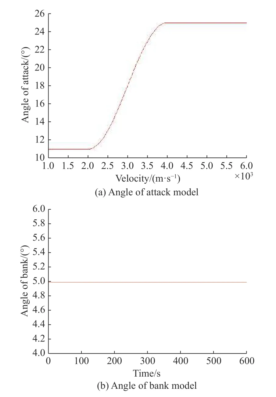
Fig. 4 Angle of attack model and angle of bank model

Assume that there is no ground cover during target detection and tracking (this paper uses the interacting multiple model (IMM) for tracking). The sensors detect elevation angles of 0° to 90° and azimuth angles of 0° to 360°.The simulation trajectory and observation information are shown in Fig. 5.

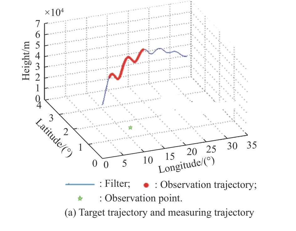
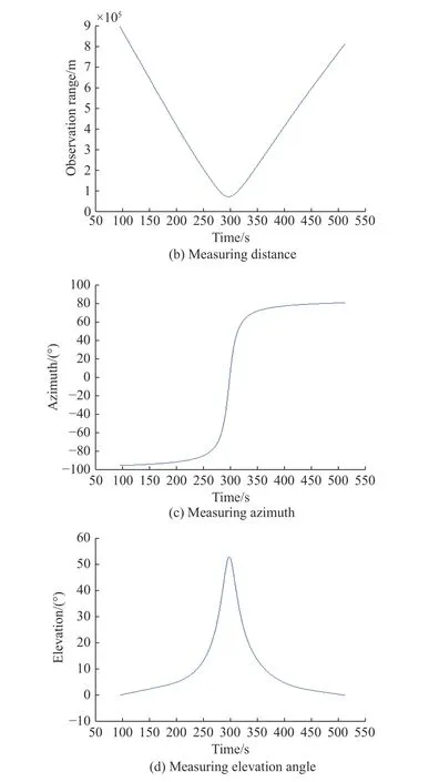
Fig. 5 Sensor measuring information

We set three different experiments. Experiment 1 is one-time tracking filtering and prediction. Experiment 2 and Experiment 3 are multiple prediction experiments, to discuss the prediction results under different tracking data lengths. In addition, the spatial distribution of prediction errors is analyzed.

5.2 Experiment 1: single trajectory prediction (data selection 200−400 s)

One-time tracking filtering and trajectory prediction are performed to verify the effectiveness of the algorithm.The prediction point is 400 s, and the tracking data from 200 s to 400 s are intercepted. The position, velocity and aerodynamic acceleration error of the target tracking in Experiment 1 are shown in Fig. 6, where RMSE denotes root-mean-square error.

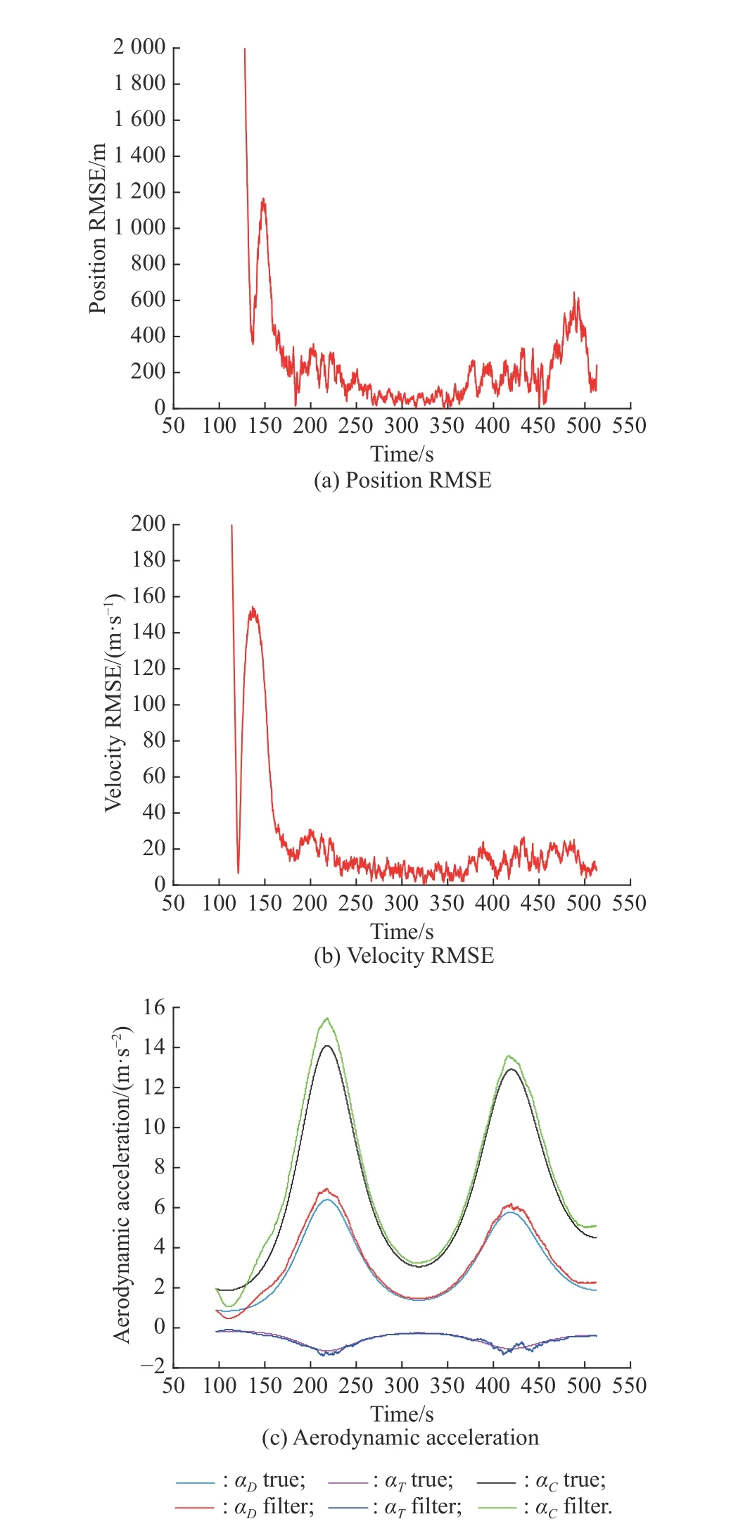
Fig. 6 Filter results

According to the step of the EMD, the following IMF results can be obtained.

As shown in Fig. 7, the overall energy of the IMF is relatively small. In which the low-frequency IMF has severe flying wing phenomenon at the data endpoints (as shown in Fig. 7(a), the end point of IMF4, and Fig. 7(b),the start point of IMF6). While the local oscillation amplitude is relatively large for the high-frequency IMF.

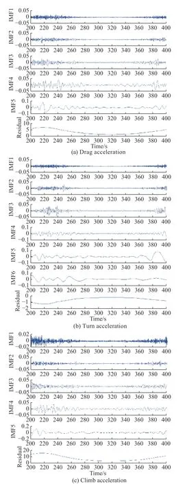
Fig. 7 EMD decomposition result of aerodynamic acceleration

The residual term and aerodynamic acceleration have similar trends (residual energy is larger), and its flying wing at the end point is smaller, which is conducive to achieving the aerodynamic acceleration prediction. According to the experimental results, the energy of the residual terms of the acceleration of drag, cornering force and climbing force has exceeded 95% of the total energy. Therefore, we directly use the residual terms as training data to perform the aerodynamic acceleration fitting and prediction. The results of aerodynamic acceleration prediction are as follows.

As shown in Fig. 8, Within 250-400 s, the error between the prediction curve and the true curve is relatively stable as a whole, but the error is larger at the peak and valley points. Especially for the acceleration of the climbing force after the prediction point, as shown in Fig. 8(e),the predicted value deviates greatly from the true value near the 470 s position.

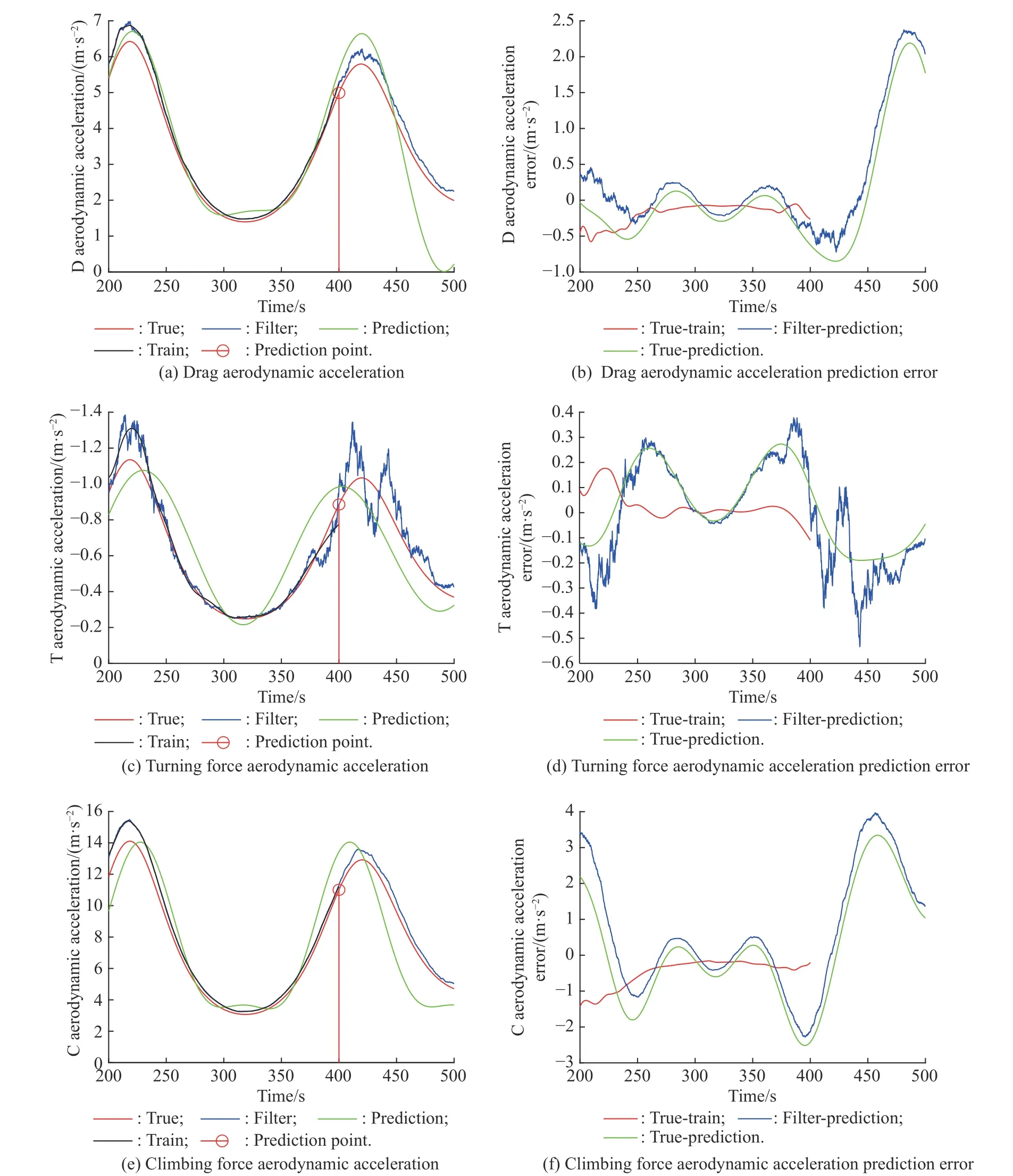
Fig. 8 Aerodynamic acceleration and prediction error

The reason is speculated as follows:

(i) The magnitude of the acceleration of the climbing force is large, and the data density of the peak point at 470 s changes greatly, resulting in a large prediction error.

(ii) We intercept the data for 200-400 s to predict the data for 400-500 s. The resonance frequency may be mismatched.

In general, from 200 s to 400 s, the three kinds of acceleration fitting errors fluctuate at the 0 position. For 400 s to 500 s, the prediction error obviously fluctuates to a large extent near the peak acceleration point, that is, the valley point of the target height. Based on this, the target trajectory is predicted, and the distance and velocity prediction errors are obtained as shown in Fig. 9.

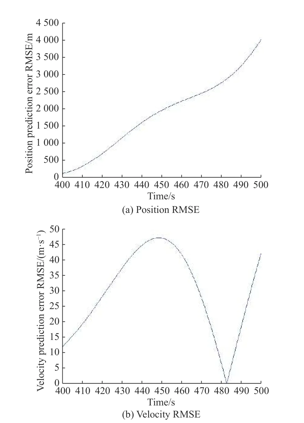
Fig. 9 Position and velocity predication RMSE

In Fig. 8, the train curve represents the data used for fitting after the clustering of sub-items. Since the energy of the residual term exceeds 95%, the train curve of each aerodynamic acceleration is the corresponding EMD residual term. As shown in Fig. 9, for the position error RMSE,it shows a roughly linear growth trend with a maximum error of about 5 km.

In terms of the speed prediction RMSE, turning force and climbing force acceleration only change the speed direction, not the speed value. Therefore, the correspondence between the drag acceleration error and the speed prediction error can be analyzed. In 400-450 s, the drag acceleration crosses the zero point, causing the speed prediction error RMSE to increase first and then decrease.After 450 s, the prediction error of drag acceleration is always greater than 0, which causes the speed prediction error to increase in the opposite direction. The maximum error is about 50 m/s. In fact, after 450 s, the error first decreases to 0 and then rises rapidly since RMSE takes the absolute value of the error.

5.3 Experiment 2: multiple trajectory prediction(data selection 200−400 s)

Perform multiple tracking and predictions (Monte Carlo number is 100). As shown in Fig. 10, the true trajectory and the predicted trajectory in 400-500 s are shown by the red and green curves, respectively. The corresponding spatial distribution of prediction error at 450 s and 500 s is shown in Fig. 11.

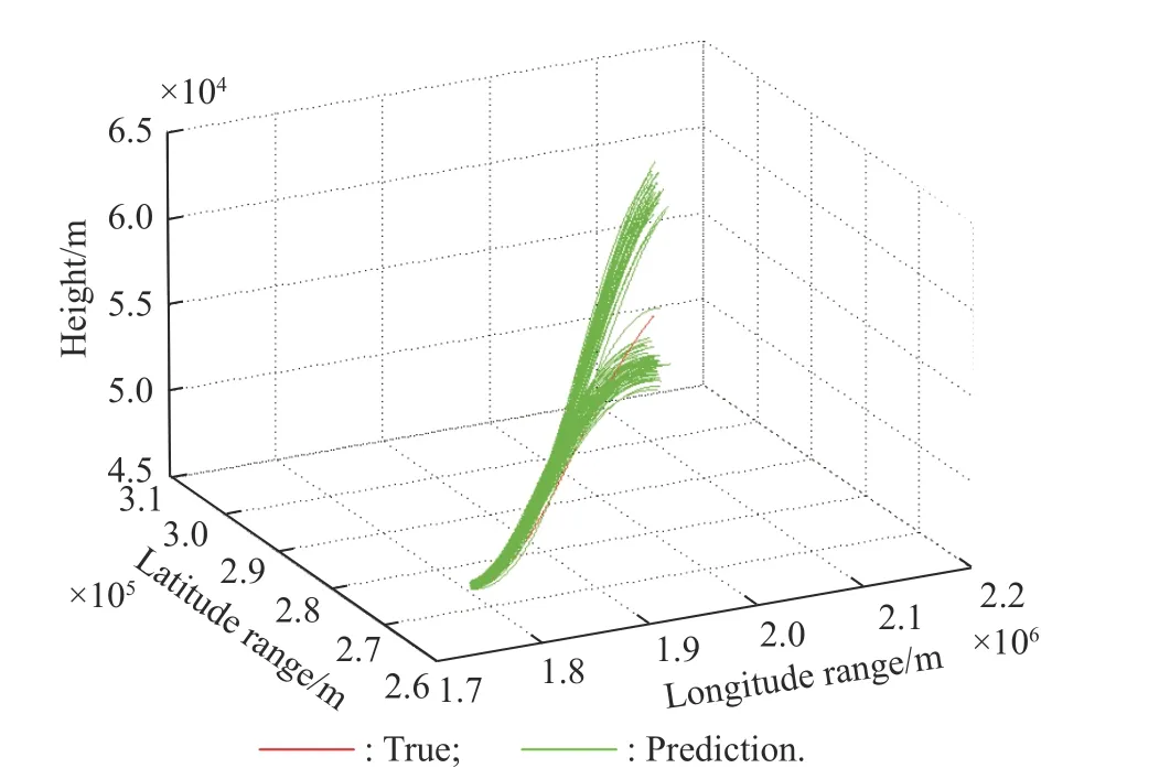
Fig. 10 Prediction trajectory cluster

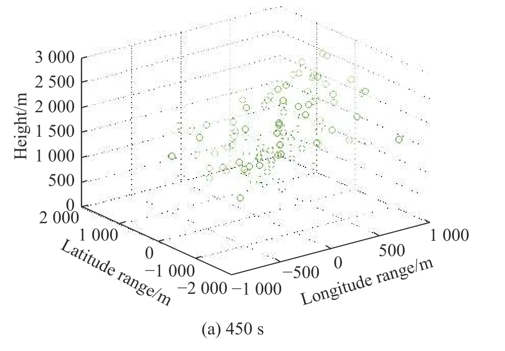
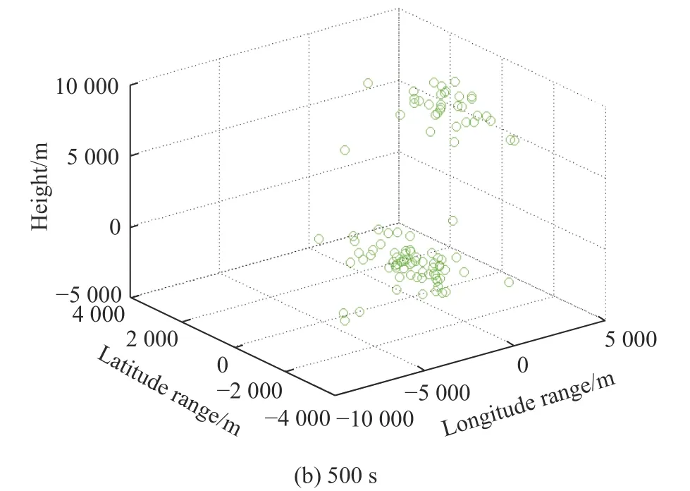
Fig. 11 Spatial distribution of trajectory prediction error

It can be seen from Fig. 12 that the error curves of the x direction and the y direction are relatively uniform,while the error distribution in the z direction after 450 s is clearly divided into two trends.

Correspondingly, at 450 s in Fig. 11(a), the spatial distribution of errors is relatively uniform, while at 500 s in Fig. 11(b), the error distribution in the height direction has a certain tendency.

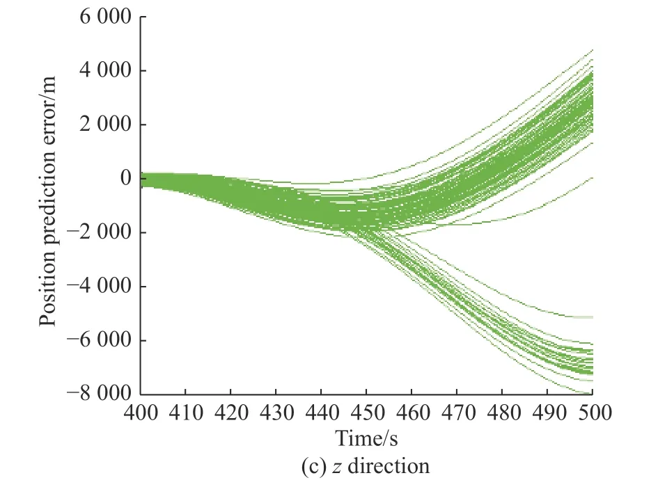
Fig. 12 Position predication error in different directions in measurement ENU coordinate system

5.3.1 Height prediction error distribution analysis

The reason for the uneven height error distribution is that there is a clear predicted trend for the acceleration of the climbing force. The prediction result of the aerodynamic acceleration is shown in Fig. 13. As shown in Fig. 13(a)and Fig. 13(b), the predicted curve distribution of drag and turning force acceleration is relatively uniform.

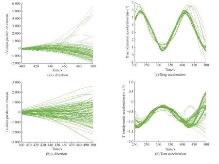
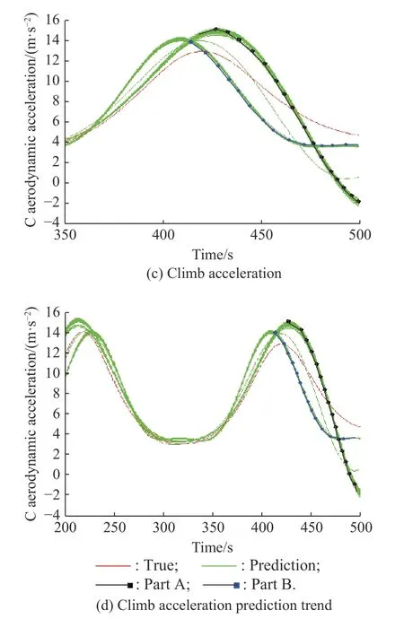
Fig. 13 Aerodynamic acceleration prediction

However, in Fig. 13(c), the predicted acceleration curve of the climbing force has a significantly different trend.The predicted trends are shown in Fig. 13(d), which are labeled Part A and Part B. Furthermore, Part A and Part B correspond to the two part error curves from the bottom to the top in Fig. 13(c), respectively.

For Part A, it intersects with the true value of the climbing force acceleration around 470 s. Therefore, the bottom error curve in Fig. 12(c) increases first and then flattens later.

For Part B, its intersection with the real value is around 420 s. Thus, the top error curve in Fig. 12(c) increases first, and after Part B crosses the true value, the error in the z-direction reverses to zero.

This is why the height error distribution in Fig. 12(c) is uneven.

5.3.2 Climb acceleration prediction trend analysis

As shown in Fig. 13, the predicted acceleration curves of drag and turning force are evenly distributed, while the predicted acceleration curves of the climbing force are divided into two types of trends. The possible reasons for this are as follows.

First, the acceleration of the climbing force is relatively large compared to the other two parameters, and the acceleration is fitted and predicted. Therefore, there are some differences in the prediction results.

Second, the data density of the acceleration of the climbing force at the peak and valley points is very different, and there may be different harmonic components.The basis function allows two similar frequency components, corresponding to the prediction results of Part A and Part B in Fig. 13(d).

5.3.3 Prediction RSE and RMSE analysis

As shown in Fig. 14, the position and velocity prediction root squared error (RSE) show an upward trend with time.The position RSE is generally distributed within 8 km,while the speed RSE is distributed within 80 m/s. The position RMSE is within 5 km and the speed RMSE is within 60 m/s.

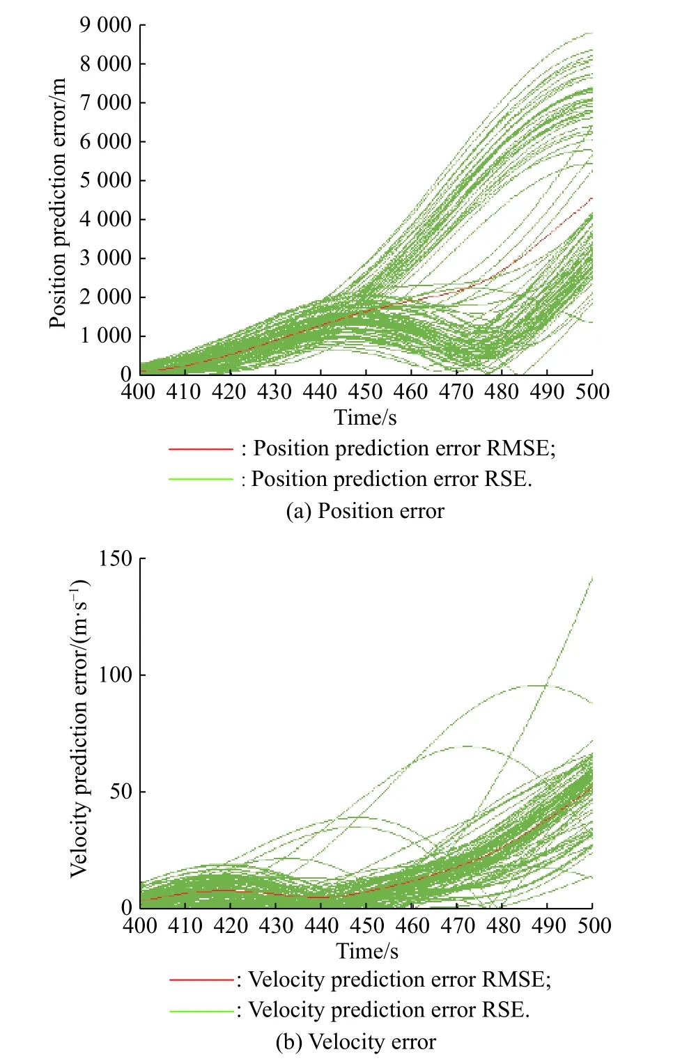
Fig. 14 Position and velocity prediction RSE and RMSE when selecting data within 200−400 s

RSE is the error square root value, and RSE is consistent with RMSE when conducting a single experiment. In 100 Monte Carlo experiments, the RMSE can only reflect the final error average, and we also pay attention to the error distribution. Therefore, the RSE and RMSE graphs are plotted at the same time to analyze the mean and overall distribution of errors.

5.4 Experiment 3: multiple trajectory prediction(data selection 120−400 s)

The tracking data of 120-400 s are selected to perform the multiple trajectory prediction, and the results are shown in Figs. 15-18.

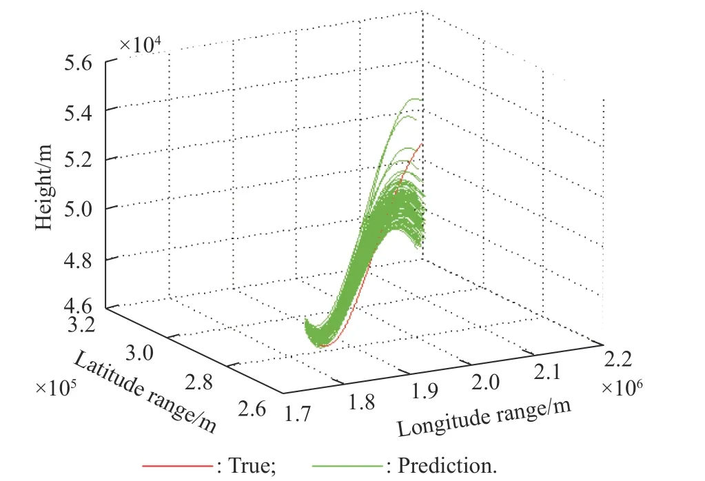
Fig. 15 Prediction trajectory cluster

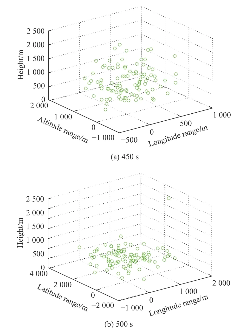
Fig. 16 Spatial distribution of trajectory prediction error

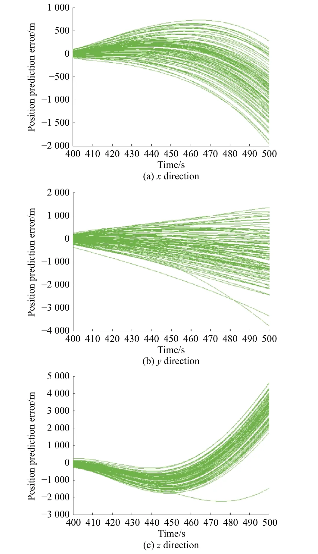
Fig. 17 Position prediction error in different directions in measurement ENU coordinate system

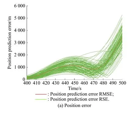
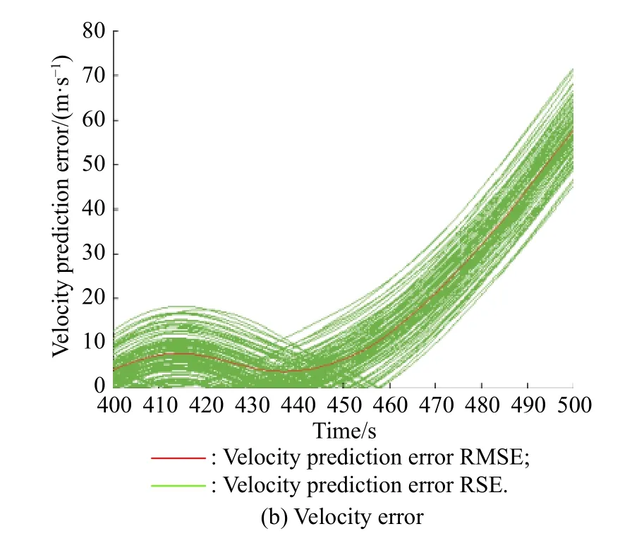
Fig. 18 Position and velocity prediction RSE and RMSE when selecting data within 120−400 s

After multiple tracking and the trajectory prediction,comparing Experiments 1-3, we can do the following analysis:

(i) In Experiment 2, the height prediction errors are non-uniformly distributed. It is shown that when aerodynamic acceleration is used as the prediction parameter,there are different trends in the prediction of the acceleration of the climbing force as shown in Fig. 13(d), which leads to uneven distribution of the altitude prediction error.

(ii) The length of training data is not positively related to the effect of the trajectory prediction. Within a certain range, appropriately increasing the data length can more accurately describe the target’s motion characteristics.However, nothing is absolute, when the data length is too long, the data that are too stale may not match the current motion pattern, which will affect the prediction effect.

Compare Experiment 2 and Experiment 3. For the position prediction error, before 450 s, Experiments 2 and Experiment 3 RSE have similar error distributions. After 450 s, the RSE of Experiment 2 is divided into two parts,but the RMSE in the two Experiments is similar.

From the perspective of speed prediction error, the difference between the two experimental results is small.Therefore, the essence of intercepting data length affecting prediction performance lies in whether more useful information can be obtained.

(iii) The NSHV flight altitude is concentrated at 30 km to 80 km, which limits the value range of the prediction error at altitude. Even if the future altitude of the target is set directly to 50 km without using a complicated prediction algorithm, the prediction error will not exceed 40 km.Whether this can indicate that the difficulty of the NSHV trajectory prediction is not in the height direction but in the range and traverse directions. As we all know, the range and traverse direction of NSHV can reach more than 1 000 km, which indicates that the prediction error interval in these two directions is much larger than that in the height direction when the prediction time is long enough.However, in a short time, according to the prediction results of this paper, the height direction prediction is close to the order of magnitude of the other two directions, or even slightly larger.

Therefore, it is not rigorous to say that the difficulty of the prediction is not in the height direction. When the prediction time is long, the prediction error of range and traverse is far more than 40 km or even hundreds of kilometers. The trajectory prediction in this case is a largescale prediction of combat intention or strike direction.However, this paper is dedicated to short-term forecasting, and its purpose is to provide support for intercepting guidance and pre-warning information firepower transfer.Its prediction error magnitude is generally in the order of tens of kilometers, and prediction errors in different directions can reach this error magnitude.

For short-term prediction or high-precision prediction,it is difficult to distinguish the prediction accuracy of different directions. The height direction prediction error is even slightly larger than the other two directions in this paper.

For the rough prediction of long-term prediction, strike intention or strike direction, the prediction error in the height direction is limited to a certain range, and its prediction is relatively easy.

6. Conclusions

In this paper, a trajectory prediction method based on aerodynamic acceleration EMD decomposition is proposed. This method first analyzes the motion characteristics of NSHV and verifies that the aerodynamic acceleration has a stable rule. On this basis, the EMD is used to decompose the aerodynamic acceleration into multiple subitems and aggregate the sub-items with similar characteristics. In order to realize the prediction of aerodynamic acceleration, a basis function is set according to its stability rule to fit and predict the future state of aerodynamic acceleration. Thereafter, the system of motion differential equations is driven by the prediction data of aerodynamic acceleration to predict the target trajectory. Finally,we validate the effectiveness of the proposed method through a series of implementations and the performance of the prediction algorithm is analyzed.