Assessment of faunal communities and habitat use within a shallow water system using non-invasive BRUVs methodology

Henriette M.V.Grimmel,Robert W.Bullok,Simon L.Deman,Tristan L.Guttrige,Mark E.Bon

aBimini Biological Field Station Foundation,South Bimini,Bahamas

bHull International Fisheries Institute,University of Hull,Hull,HU6 7RX,United Kingdom

cIndependent Researcher,San Carlos,CA,USA

dDepartment of Biological Sciences,Florida International University,3000 NE 151th Street,North,Miami,FL,33181,USA

eSaving the Blue,Kendall,Miami,33186,USA

ARTICLEINFO

Keywords:

Baited remote underwater video

MaxN

Mangrove edge habitat

Bahamas

Bimini

ABSTRACT

Seagrass and mangrove habitats have long been established as critical for diverse species at various life-stages,particularly as nursery grounds.However,despite their intrinsic and environmental value,these ecosystems are increasingly threatened by anthropogenic activities.In Bimini,Bahamas,where ongoing development threatens ecosystem integrity,baited remote underwater video surveys(BRUVs)were used to examine faunal communities in both nearshore habitat and a shallow water central lagoon(average depth 1 m).The study assessed species abundances and spatial distribution in a currently unperturbed of the North Bimini Marine Reserve(NBMR).

A total of 140 BRUVs,conducted over a 13-month period,recorded 62 species from 27 different families.MaxN was used to assess relative abundances and multivariate analyses(i.e.nMDS,PCA,PERMANOVA)investigated differences in community composition across discrete factors and environmental variables.Boosted Regression Trees(BRTs)were used to explore environmental variables for their uncorrelated influences on recorded species diversity.Findings evidenced the importance of habitat diversity and particularly mangroveadjacent habitat for teleost fishes in Bimini with species diversity and abundance being significantly greater in the mangrove-adjacentdge habitat.Further,the study highlighted differences in environmental conditions between habitat types and the association this had with species diversity,abundance and distribution.Despite the shallow water environment,BRUVs served as a scalable,non-invasive technique to assess community structures within the study site.Results from this study should inform ongoing decision-making processes regarding the protection of the Bimini Islands ecosystem.

1.Introduction

Mangrove forests are one of the most productive systems known in the marine environment.They play a fundamental role in carbon sequestration(Alongi&Mukhopadhyay,2015;Hutchinson,Manica,Swetnam,Balmford,&Spalding,2014;Siikamäki,Snachirico,&Jardine,2012),helping to mitigate climate change on a large-scale,while serving as essential habitat for a diverse range of fish and macroinvertebrate communities in tropical and temperate zones(Kathiresan&Bingham,2001;Lugendo,Nagelkerken,Kruitwagen,van der Velde,&Mgaya,2007;Newman,Handy,&Gruber,2007;Valiela,Bowen,&York,2001)on a small-scale.These systems are of notable importance to species throughout juvenile development stages,as they provide abundant food resources and refuge from predators(Guttridge et al.,2012;Heupel,Carlson,&Simpfendorfer,2007;Newman et al.,2007)and thereby promote and support recruitment into adult populations in surrounding habitats(Gillanders,Able,Brown,Eggleston,&Sheridan,2003;Mumby et al.,2004;Nagelkerken et al.,2001).Despite their known economic,ecological and social value(Alongi,2008;Costanza et al.,1997;Siikamäki et al.,2012),loss and degradation of global mangrove areascontinue atalarming rates(Knip,Heupel,&Simpfendorfer,2010;Miththapala,2008;Murdiyarso et al.,2015;Polidoro et al.,2010;Valiela,2001)making mangroves one of the most threatened coastal,marine habitat types(Valiela,2001).Seagrass habitats are not faring much better and are also under threat(Orth et al.,2006;Waycott et al.,2009).Despite this,in many parts of the world,sufficient protection of mangroves,and related environments,is lacking.Pervasive human influence on the marine environment has long been a topic of concern(Giakoumi et al.,2015;Halpern et al.,2008;Pauly,Christensen,Dalsgaard,Froese,&Torres,1998;Stevens,Bonfil,Dulvy,&Walker,2000;Worm et al.,2013)and many marine ecosystems,including mangroves,face a constantly increasing number of anthropogenic disturbances that have the potential to negatively affect their function and dynamics(Henson et al.,2017;Stelzenmüller,Lee,South,&Rogers,2010)and threaten species extinctions(Brook,Sodhi,&Bradshaw,2008;Tilman,May,Lehman,&Nowak,1994).

Consequently,mangroves are listed under a range of international treaties(e.g.Convention on International Trade in Endangered Species of Wild Fauna and Flora(CITES),the RAMSAR Convention,Convention on Biological Diversity(CBD)),some of which the Bahamas are signatory to(Buchan,2000).However,these treaties offer only limited protective value.Most mangroves are poorly represented in protected areas(Polidoro et al.,2010)despite their connectivity to other marine ecosystems(i.e.seagrass communities,coral reefs)(Mumby et al.,2004;Nagelkerken et al.,2001,2002;Sheaves,Baker,Nagelkerken,&Connolly,2015).Understanding the ecological functioning and connectivity of natural systems is essential and monitoring faunal communities to understand their habitat requirements may inform effective management,the consequences of degradation,and help conserve healthy marine habitats(Cabello et al.,2012;Katsanevakis et al.,2012;Rosenberg,Bigford,Leathery,Hill,&Bickers,2000).Demersal fishes,for example,play an important role in the maintenance of most ecosystems(Hardinge,Harvey,Saunders,&Newman,2013)and express strong relationships with their local environment(Chat field,Van Niel,Kendrick,&Harvey,2010).Nevertheless,little is known of the factors that influence fish habitat use patterns and associated habitat requirements(Sims,2003).

The Bimini Islands in the Bahamas are largely fringed by red mangrove(Rhizophora mangle)forests and adjacent seagrass beds,and known to be an important nursery habitat for lemon sharks(Negaprion brevirostris)(Feldheim,Gruber,&Ashley,2002;Gruber et al.,1988;Heupel et al.,2007).While research on the lemon shark has been ongoing for over two decades(e.g.Feldheim et al.,2014),little is known about abundance and distribution of faunal communities as a whole.Only one invasive study,conducted over a decade prior to this research,has been undertaken(i.e.Newman et al.,2007).

Over the last 20 years,intensified resort development on North Bimini has resulted in large areas of mangrove removal as well as dredging and sediment dumping activities(Gruber&Parks,2002;Jennings et al.,2008,2012;Trave&Sheaves,2014),culminating in a loss of at least 39% of mangroves in the area(DiBattista,Feldheim,Garant,Gruber,&Hendry,2011;Jennings et al.,2008).A North Bimini Marine Protected Area(MPA)was proposed as early as the year 2000 by the Bahamian government(Gruber&Parks,2002;Wise,2014).Boundaries were de fined and the North Bimini Marine Reserve(NBMR)declared in 2009,but the MPA remains unimplemented to date,with further development ongoing or planned(Fuentes et al.,2019).

In this study,Baited Remote Underwater Video surveys(BRUVs)were used to survey the abundance,composition and spatial distribution of faunal communities within the mangrove-fringed,sandy seagrass lagoon site connecting the north and south islands in Bimini,Bahamas,an area not yet impacted by development and largely encompassed by the delimitations of the proposed marine reserve.

BRUVs offer a minimally invasive,cost-effective means of measuring abundance,sampling a wide range of species with a greater statistical power than most other methods(Harvey,Cappo,Butler,Hall,&Kendrick,2007).Consequently,interest in research using BRUVs has grown rapidly and many studies have used this methodology to assess the composition of marine species assemblages(e.g.Cappo,Speare,&De’ath,2004;Clarke,Whitmarsh,Fairweather,&Huveneers,2019;De Vos,Gotz,Winker,&Attwood,2014;Harvey et al.,2007;Whitmarsh,Fairweather, & Huveneers,2017;Whitmarsh, Huveneers,&Fairweather,2018)some focusing on particular family groups,like elasmobranchs(Brooks,Sloman,Sims,&Danylchuck,2011;Sherman,Chin,Heupel,&Simpfendorfer,2018).However,only a few studies have utilised BRUVs methodology in shallow-water environments,pertaining to depths＜5 m(e.g.Whitmarsh,Fairweather,Brock,&Miller,2014;Gilby,Tibbetts,Olds,Maxwell,&Stevens,2016;Kiggins,Knott,&Davis,2018;Jones,Cullen-Unsworth,Howard,&Unsworth,2018).

The main objectives of this study were to:1)evaluate BRUVs as an adequate methodology to document community structures in very shallow(av.depth 1 m)mangrove-adjacent seagrass and sandy environments;2)record the diversity of marine fauna(to species level where possible)that use the study site,identifying their spatial distribution and relative abundance;and 3)determine which/if any discrete or environmental factors influence distribution,relative abundance and composition of faunal groups.

2.Materials and methods

The Bimini Islands,north and south Bimini,(25°44′0.9” N,-79°16′23.0”W)are located on the north-western edge of the Great Bahama Bank,roughly 86 km east of the coast of Miami,Florida(USA).This study was conducted on the eastern side of the north island,with a site known as Bone fish hole at its most northern tip and the adjacent lagoon area to its south and east(Fig.1)(Edrén&Gruber,2005;Morrissey and Gruber,1993b).The study site encompasses the southern,currently unperturbed by development,portion of the proposed NBMR.

2.1.Data collection

Deployment locations were selected randomly using the‘create random points’function in ArcGIS,after Cappo et al.(2004)and Bond et al.(2012).Previously undertaken depth profiling of the lagoon identified exact delimited areas that would allow sampling within the study site at different tidal phases(H=high,L=low).Tidal phases and states(F=falling,R=rising,S=slack)were adopted from the National Oceanic and Atmospheric Administration(NOAA)tides and currents database(NOAA,2014).The minimum distance between simultaneously deployed BRUVs was 1 km to eliminate bias of overlapping chum slicks.Deployment locations were grouped according to their distance from the shoreline,reflecting known changes in species richness and distribution across different habitat types(Field et al.,1998;Nagelkerken et al.,2001;Jones,Cullen-Unsworth,Howard,&Unsworth,2018)Habitat type was thus de fined:Mangrove Edge(ME:0–50 m from the shoreline)and Open Lagoon(OL:＞ 50 m from the shoreline)(after Newman et al.,2007).

BRUV rigs were constructed of steel reinforcing bars arranged in a pyramid shape for stability and welded together to create a 60×60 cm base,with a total height of 87 cm.A GoPro Hero(2nd edition)camera in an underwater housing was attached to the frame,positioned 40 cm above the seabed level and with a sunshield for glare reduction placed above it.The bait cage(dimensions:20 x 14×16 cm)was positioned on a rebar arm extending a distance of 100 cm from the camera mount and contained a standardized 800g(frozen weight)of crushed Atlantic menhaden(Brevoortia tyrannus)(Fig.2,after Harvey et al.,2007).The bait was placed in chum bags to avoid fast dispersal.Prior to deployment,it was defrosted completely to ensure standardised conditions of the bait throughout the series of deployments.

Each BRUV was deployed for 70 min,of which the first 10 min was considered ‘settling time’and excluded from analysis.A soak time of 60 min was deemed sufficient to allow for the greatest number of species and individuals possible to appear within the frame(Watson,Harvey,Fitzpatrick,Langlois,&Shedrawi,2010).The time of deployment was de fined by the tidal phase and state,and deployments were set to record either in the hour before or after maximum high or minimum low tide to encourage the greatest dispersal of the bait plume.Sample locations were navigated to with a flat-bottom skiffand handheld Global Positioning System(GPS)(Garmin Ltd,GPS 72H).Upon arrival,environmental parameters(temperature[oC],salinity[ppt]and dissolved oxygen(DO2)[%])were measured with a YSI Pro2030(YSI Inc.OH,USA).Depth was measured to the nearest centimetre with a marked stick and horizontal visibility was recorded with a tape measure,Secchi disk(diameter 22 cm),and snorkeler at the surface,as depth never exceeded 3 m.Flow velocity(cm.s-1)and direction were measured using a flow meter with a low velocity paddle(General Oceanics,Florida,USA),and a compass and soluble dye respectively.BRUVs were then positioned to record down current,in accordance with the predominant tidal state,to maximise the likelihood that any animal attracted to the bait would approach the apparatus within the camera's field of view,thereby increasing the accuracy of the abundance estimates.Once recording began,the team moved several kilometres away from the deployment site to minimize disturbance.Upon retrieval,the aforementioned environmental parameters were again recorded.The seagrass coverage was estimated on site using a quadrat(105×105 cm containing twenty- five 20×20 cm sections)along a 20 m transect line moving outward with the direction of flow.It was visually determined to the closest 5%.

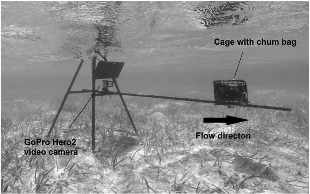
Fig.2.Frame used for BRUVS with chum bag and bait cage(right)and video camera ready to record at beginning of a deployment.A dark sunshield was fixed above the camera to reduce glare of the sun and water reflection for the video recordings.

2.2.Video analysis

Videos were analysed in real-time using VLC Media Player(v.2.1.3,www.videolan.org/vlc),by experienced observers.While watching the recording,the maximum number(MaxN)of individuals of a family or species present in any one frame or passing through a video segment of 30–60 s(after Cappo,Harvey,Malcolm,&Spears,2003)was documented.MaxN is a commonly used index for relative abundance in the analysis of fish assemblages(Brooks et al.,2011)and is considered a deliberately conservative estimate of true abundance(Cappo et al.,2003;Gutteridge,Bennett,Huveneers,&Tibbetts,2011).The maximum number of individuals(MaxI)was used in case of elasmobranchs,where individuals could clearly be identified as distinctly different animals(Bond et al.,2012).Individuals were taxonomically identified to family and,where possible,to species levels.Unidentifiable individuals,due to distance from the camera or turbidity,were excluded from further analysis.

2.3.Data processing and analysis

The discrete factors that were used for analysis were tidal phase(H,L),season(wet season–November to April;and dry season–May to October),and habitat type(ME and OL).Environmental variables(temperature(°C),salinity(ppt),visibility(m),percentage seagrass coverage(%),flow velocity(cm.s-1),dissolved oxygen(%)and depth(m))were averaged for each sample,using the prior and post deployment values,and then tested for normality,using the Shapiro-Wilk test in R(v.3.0.2)(R Development Core Team,2008).Except for average temperature(p＜0.05)none of the other abiotic factors were normally distributed(p＞0.05).A student t-test and a Wilcoxon Rank Sum test were then used,respectively,to test for significant differences of these variables across discrete factors(i.e.habitat type,season,tidal phase)in R.

2.4.Ecological data analysis

Abundance,MaxN,and environmental data were explored using multivariate analyses with the PRIMER(v.6)program and its PERMANOVA extension pack(Anderson&Walsh,2013;Clarke&Gorley,2006).PRIMER procedures are highly robust,producing easily interpretable outputs because ordinations and tests are generated through permutation of the data,making very few assumptions about the distribution and form of the data(Anderson,Gorley,&Clarke,2008).The program has been used to interpret marine species assemblage data in various studies(e.g.De Vos et al.,2014;Hardinge et al.,2013;Santana-Garcon,Newman,Langlois,&Harvey,2014;Whitmarsh et al.,2018).Environmental data were normalized to allow for the construction of a Euclidian distance resemblance matrix,whereas the MaxN and MaxI abundance data were subjected to a square root transformation to reduce variance heterogeneity and the influence of highly abundant species(Gutteridge et al.,2011;Hardinge et al.,2013).A Bray-Curtis similarity index was then used on the transformed biological data to create a triangular similarity matrix(Clarke& Warwick,2001;Hardinge et al.,2013).The resulting matrix for similarity of faunal composition was then plotted using non-metric multidimensional scaling(nMDS),giving information on spatial variation.This was done for abundance data by family and species across the three discrete factors.Resulting from this,community composition was further investigated using a 2-way permutational multivariate analysis of variance(PERMANOVA).Similarity percentages(SIMPER)were then derived to determine which families contributed most to differences across factors.A Principal Component Analysis(PCA)was used to visualize any patterns within the environmental data,displaying vectors for each environmental variable.Differences between these data were also tested using PERMANOVA with habitat type and tidal phase as factors.Spatial variation in abundance of different faunal groups was visually examined and mapped using the GPS information of each deployment location and corresponding MaxN values in ArcGIS V.10(ESRI,2011).Furthermore,Shannon-Wiener(SW)diversity indices(H'ln)were calculated for the datasets of abundance,at family as well as species level,using PRIMER.Differences in H'ln across habitats were then also tested with a Wilcoxon Rank Sum test.

2.5.Boosted regression tree analysis

Multivariate regression trees are used as a form of meta-analysis,for example to determine environmental data that highly influence faunal assemblage dynamics or structure(Horta e Costa et al.,2014).As a more complex form thereof,boosted regression trees(BRTs)identify the combination and relationships of explanatory variables that best describe variations in the response variable(Elith,Leathwick,&Hastie,2008).They are useful for the analysis of continuous response variables while being better adapted to dealing with non-linearity and interactions of explanatory variables and factors(Zuur,Ieno,&Smith,2007).Their use in marine ecology is increasing(Dedman,Officer,Brophy,Clarke,&Reid,2015;Froeschke&Drymon,2013;Froeschke&Froeschke,2011)as they deal with missing values,outliers,multicollinearity,numerous explanatory variables and data-poor situations well(Elith et al.,2006;Loos,2006;Vincent et al.,2004).

Temperature,salinity,visibility,seagrass cover,depth,flow velocity,tidal state and phase,month,habitat type and dissolved oxygen were used as explanatory variables in the beginning.The response variables were chosen upon preliminary BRT results,whereby total MaxN(of all families/species across all BRUVs)and MaxN of non-teleost groups were excluded due to poor representation of the community composition and not being data-rich enough for multiple runs,respectively.Results of preliminary BRTs using all available explanatory variables also informed the selection of explanatory variables for the final models.Uninformative,non-contributory,or inherently auto-correlated variables(i.e.season)were discarded,whereas tidal phase and tidal state where combined into one single variable to improve precision.The BRT methodology followed the framework set out in(Dedman,Officer,Clarke,Reid,&Brophy,2017),with explanatory and response variables as detailed in Table 1.

The highly data-sparse nature of BRUVs can mean BRTs resolve quickly but with potentially unreliable outputs(the First Impressions Count problem(Dedman,2017)).Gbm.loop was therefore used to mitigate against implausible results that might arise from single-run BRTs by taking the averages from ten runs using the same BRT function arguments for selected response variables.All three response variables used a learning rate of 10-3(SW families and SW species)or 10-1(MaxN teleosts),a bag fraction of 0.9 and tree complexity value of 9(SW families,MaxN teleosts)or 10(SW species).Other parameters were left at their defaults.

3.Results

The BRUVs setup used for this research was effective in recording faunal assemblages across all areas of the study site,even in very shallow water.Of all deployments,97% were recordered in less than 2 m depth and 61.7% at an average depth of less than 1 m.The experimental setup performed well in all cases.Twenty-four deployments were excluded from analyses due to disturbance to the immediate site during recording(i.e.boat activity)or due to camera/battery failure.

3.1.Faunal community composition and relative abundances

A total of 140 BRUVs were deployed over 13 months(41 sampling days).Random tidal deployments resulted in 81 samples collected during low tide and 59 during high tide periods.Through video analysis,a total of 5786 individuals were observed.Of these 82.2%,4800 individuals,were identified to species level.Within the study site,BRUVs facilitated the documentation of 62 species belonging to 27 family groups(Fig.3),18 of which were teleosts consisting of 52 teleost species(Table 2).Further,three species of elasmobranchs,five species of crustaceans and two species of marine reptiles were identified(see Fig.3 for family groups).Teleost fishes comprised the most abundant family groups identified in the study site.The five most abundant family groups,all teleosts(Lutjanidae,Hemiramphidae,Carangidae,Gerreidae and Atherinidae),made up 80% of overall MaxN estimates,while the five most frequently sighted families(Carangidae,Sphyraenidae,Gerreidae,Lutjanidae and Portunidae)made up 55%.With the exception of Portunidae,no non-teleost families contributed more than 1% to total MaxN and thus,further analysis focused on teleost fish families.Lutjanidae was the most common family across all sampling,accounting for 20.5% of total MaxN and occurring in 58 of all BRUVs(41.4%).Carangidae was the most frequently sighted family,appearing in 76(54.3%)videos.Results showed that relative abundances of individual species varied greatly,from 1 to 1005 individuals,and only certain species were frequently sighted throughout the course of the study.Species that were observed in more than a third of all videos were Sphyraena barracuda(Great Barracuda),Lutjanus griseus(Grey Snapper)and Caranx ruber(Bar Jack).

3.2.Habitat preferences and spatial distribution

Overall relative abundance varied across the study site(Fig.4).Mean MaxN for ME sites was 6.5(se±0.4)whereas mean MaxN for OL sites was 4.1(se±0.2).nMDS produced a best stress level of 0.22,which is reasonable but can signify that the configuration was not a good representation of the patterns in the data.In this case,however,patterns were relatively evident and stress levels are known to increase with larger sample sizes(Clarke,1993).

PERMANOVA revealed significant differences in overall relative abundance of teleost families between habitat types(p＜ 0.01).Further,significant differences in SW indices between habitat types were found(Wilcoxon Rank Sum test,p＜0.05).ME sampling locations showed greater richness and evenness,according to the Shannon-Wiener index,than OL sites.No statistically significant differences were found in faunal abundances between different tidal phases or seasons.

The OL habitat type was found to be less similar in faunal composition across samples than the ME habitat type(SIMPER).Average similarity in family composition between OL habitat samples was 25.1% and 42% between ME samples.Eight families contributed to 90% of similarity in OL sites and nine families to that in ME locations.Sixteen familiesexplained thedissimilarity between habitatsaltogether.Carangidae contributed 28.1% to similarity of samples in OL samples followed by Hemiramphidae with 16.9% and Portunidae with 13%.In ME sites Lutjanidae accounted for a large portion of the similarity(43.1%)across sampling locations,followed by Gerreidae with 10%.

Spatial distribution maps(Fig.5)showed variability in habitatpreferences between the selected family groups,as well as quantifying differences in proportional MaxN within those family groups,across the study site.

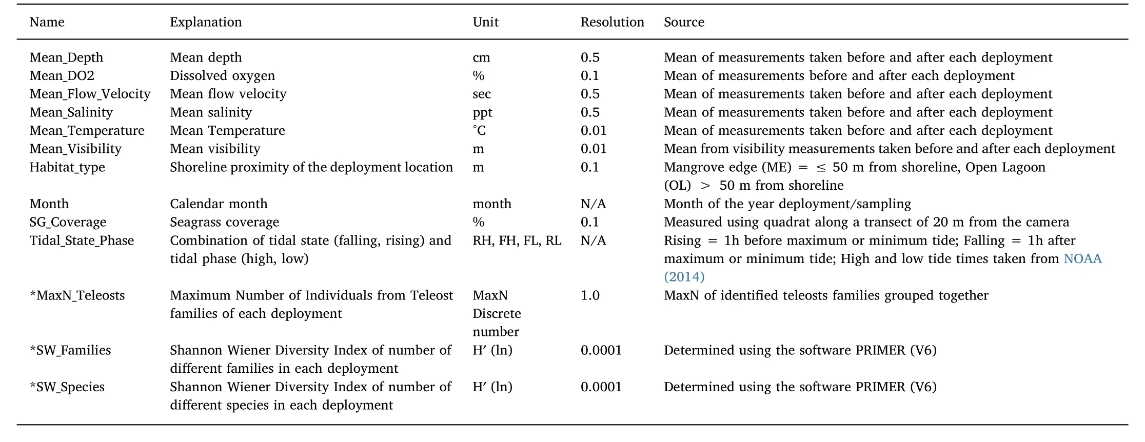
Table 1Explanatory and response variables(＊)used in boosted regression tree modelling,listed alphabetically,including unit,resolution and source.

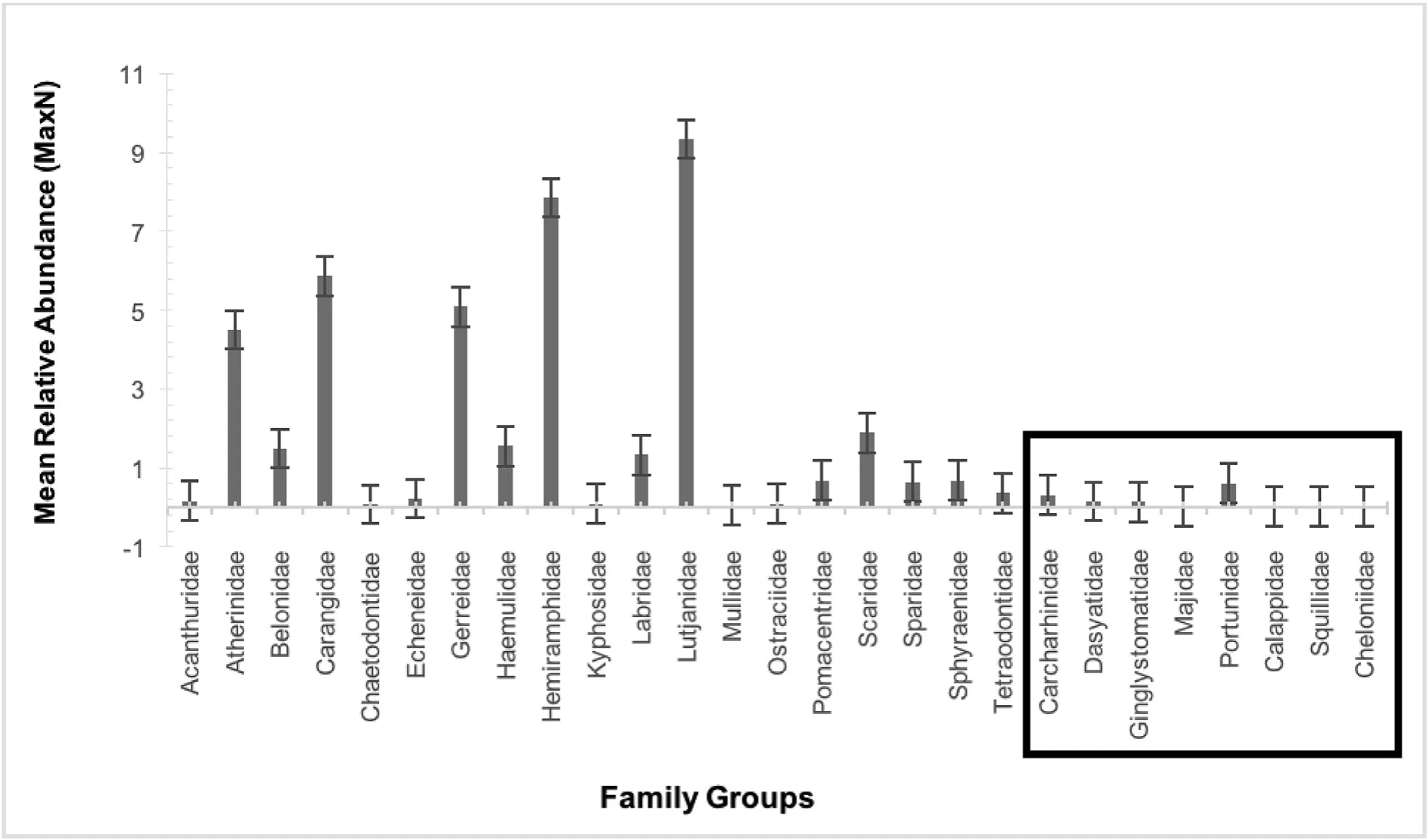
Fig.3.Mean MaxN of family groups across all BRUVs with respective standard errors;teleosts alphabetically left to right,followed by non-teleost family groups to the right().

3.3.Influence of environmental variables on community structure

Temperature showed highly significant differences when tested across seasons(student t-test,p＜0.01).All other environmental,nonnormally distributed,variables were tested across factors(i.e.habitat type,tidal phase and season)using a Wilcoxon Rank Sum Test in R(Table 3).Test results for seagrass coverage and depth were not presented,due to their strong correlation to habitat type and tidal phase,respectively,but included in the PCA and the BRT analysis.Salinity presented highly significant differences across season and visibility showed significant differences between habitat type.Dissolved oxygen was significantly different across season while flow velocity showed no significant differences across any factor.

PERMANOVA of environmental data evidenced significant differences in environmental data between habitat types across all sites(PERMANOVA,p ＜ 0.01).PCA highlighted distinct differences in mean percentage seagrass cover,which was far greater in ME areas,and in mean visibility,which was greater in OL areas(Fig.6).Differences in temperature or salinity where not distinct between OL and ME samples,whereas greater depth showed to be associated with OL habitat.Dissolved oxygen was excluded from PCA analysis due to the lack of a full dataset of this variable.

Additional features of the data were explored using BRTs which were run for three response variables(MaxN of teleosts,SW indices offamilies and species)(see section 2.5).Bar plots detailing the relative influence of explanatory variables upon the MaxN of teleosts and line plots describing these relationships,are presented in Appendix I in Supplementary Material.However,BRT results for Shannon Wiener indices of families and species were both similar and thus only those for the SW species response variable are presented.The SW index based on the MaxN of species recorded across all BRUVs is the most representative variable of the local faunal community composition in terms of providing the highest possible resolution(SW being a measure of species diversity and evenness)within this study.

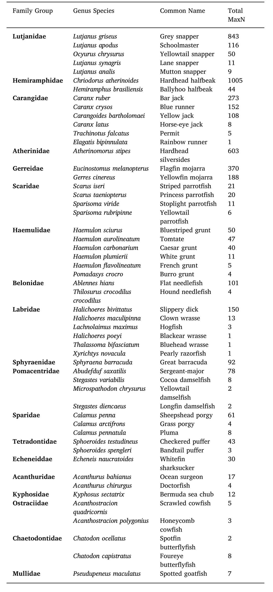
Table 2Identified teleost species with numbers of total observed individuals over the course of the study organized from highest to lowest MaxN by family within families by species from highest abundance to lowest.Genus and species name adopted from the World Register or Marine Species(WoRMS Editorial Board,2017).This representation excludes individuals that were only identified to family level.

BRT results identified a very positive relationship between species diversity and depth of 75–130 cm.Too few data was available to discern this relationship further.Seagrass coverage had a similarly positive relationship,with lowest species diversity relating to 0% seagrass coverage and rising near-linearly to highest species diversity at＞65% seagrass coverage.BRT results on mean visibility supported the association of mangrove edge habitat with high species diversity.There was a negative relationship between mean visibility increasing from 9 to 13 m,and species diversity falling simultaneously,with a specific peak of low species diversity at 9 m visibility.Results showed a noticeably positive threshold relationship between the response variable and a temperature＞31°C,as well as with rising salinity and falling and slack low tides.A negative relationship was identified between declining species diversity and rising DO2 and flow velocity,respectively.For plot details see Appendix II in Supplementary Material.

All BRT results combine to suggest that,in this study site,highest species diversity is found in areas with dense bottom coverage in the form of seagrass(＞65%),within 50 m of the mangrove fringed shoreline,or both.This relates moderately to low visibility and further,warm temperatures are best,but not when it is extremely shallow,nor when depth exceeds 130 cm.The combination of these conditions provides the best explanation for the response variable species diversity(using Shannon Wiener as the index).

4.Discussion

Although BRUVs have frequently been applied to survey species abundance and biodiversity across a broad range of geographic areas and aquatic habitats,Whitmarsh et al.(2017)reviewed 161 peer-reviewed BRUV studies,finding only a very small percentage exclusively sampling in the shallowest depth range(9 studies at≤5 m).Though other shallow water BRUV studies have more recently been published(Jones et al.,2018;Kiggins et al.,2018)methodological approaches are still developing.Here we demonstrated the application of a BRUV setup in a shallow water habitat with all samples deployed in＜3 m(semidiurnal tidal range-1–2 m,average depth 1 m).

BRUVs quantified faunal community structure through species diversity,relative abundance and spatial distribution,within a mangrovefringed lagoon,across a range of environmental conditions.Findings highlight dissimilarities in how different faunal groups use this site.

Many species,including those contributing some of the largest proportions to overall relative abundance,were found to be strongly associated with the mangrove-fringed shoreline.Many studies have investigated the value of mangrove systems and their important interactions with coastal fish communities(e.g.Jelbart,Ross,&Connolly,2007;Laegdsgaard&Johnson,1995;Robertson&Duke,1990;Sheaves,Johnston,&Baker,2016).Predation exerts a strong influence on habitat selection in fishes(Hughie et al.,1994;Munsch,Cordell,&Toft,2016;Sheaves,2005;Werner,Gilliam,Hall,&Mittelbach,1983)and mangrove prop-roots provide structural complexity,offering refuge value to juveniles and sub-adult fishes,when compared to other habitat types(Knip et al.,2010;Sheaves,2005;Stump,Crooks,Fitchett,Gruber,&Guttridge,2017).Laegdsgaard and Johnson(2001)tested predator avoidance in three habitat types(mangrove forests,seagrass beds and mud flats),showing that in controlled environments; fish immediately seek the shelter of mangroves upon introduction of predators.Alternative environmental factors,however,may also explain the observed correlations between habitat type with relative abundance and species diversity.This research suggests that the physical nature of the nearshore environment may also enhance its refuge value.Distinct differences in seagrass coverage and visibility were observed between habitat type.Overall,seagrass coverage was far greater at ME sites than in OL sites.Conversely,visibility was much higher in the sandy bottom open lagoon areas.The increased seagrass cover and associated reduction in visibility may offer a cryptic refuge for fish species.Previous research has shown macrofaunal species richness to be much higher in seagrass areas when compared to adjacent un-vegetated sites(Lee,Fong,&Wu,2001)and some fish and invertebrate species select dense seagrass areas due to habitat preference and not predator avoidance(Bell&Westoby,1986).A study on young-of-the-year pike Esox lucius suggests that low-visibility habitat can afford prey fish with a permanent level of protection against predators(Skov,Berg,Jacobsen,&Jepsen,2002).BRT results,which de-correlate variables to the extent that is possible,demonstrated associations between species diversity and depth.Such associations have been previously documented in the marine environment for teleost fishes(Smith&Brown,2002).

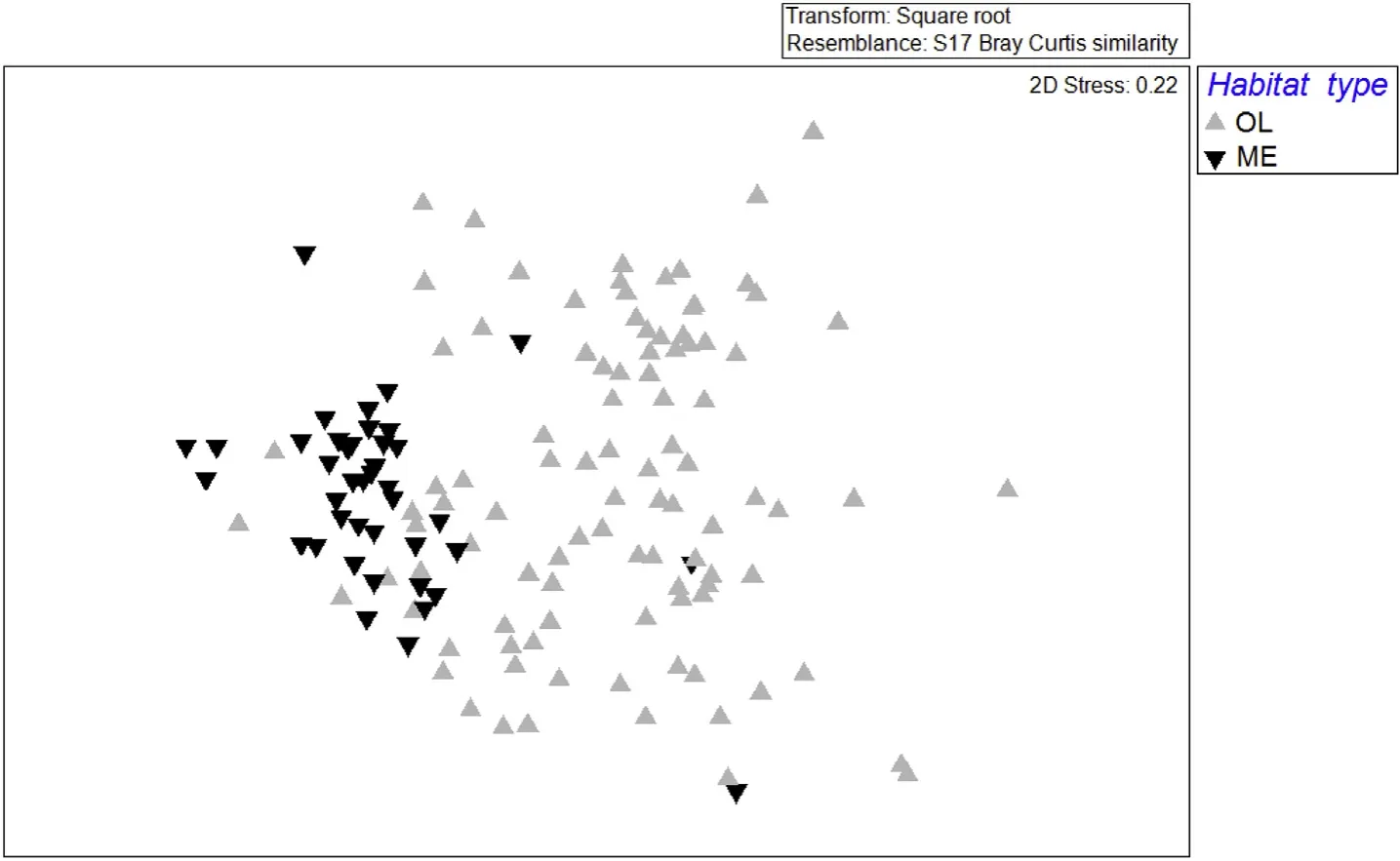
Fig.4.Non-metric multidimensional ccaling plot(nMDS)of MaxN abundance data sorted showing similarity in families across factor habitat type(ME,OL).The greater the distance between two samples,the greater the dissimilarity in families and their abundances.

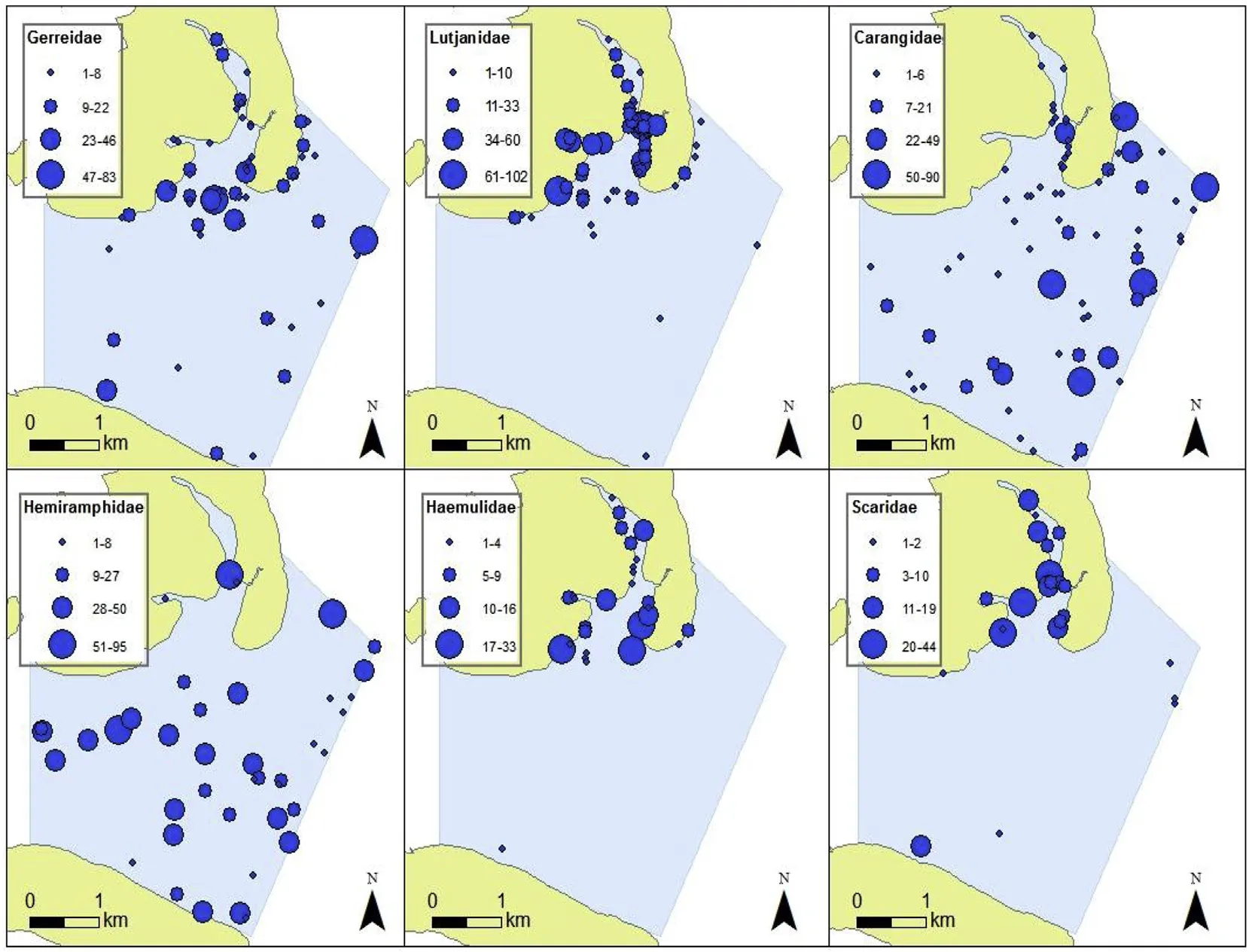
Fig.5.Distribution maps showing spatial relative abundance across the study site of the most abundant family groups consisting of more than one species each:Gerreidae(a),Lutjanidae(b),Carangidae(c),Hemiramphidae(d),Haemulidae(e)and Scaridae(f);classified with natural breaks(Jenks).The proportional symbols(blue),thus,correspond to individual legends giving the different MaxN per sampling location in which the respective family group was sighted.(For interpretation of the references to colour in this figure legend,the reader is referred to the Web version of this article.)

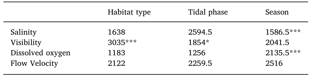
Table 3Wilcoxon rank sum test results for non-normally distributed environmental variables with Wilcoxon rank sum statistic values and significance levels.N=140 for all sets of environmental variables with exception of dissolved oxygen(N=104).

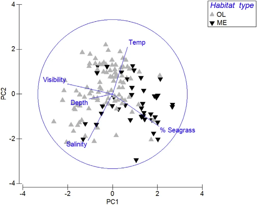
Fig.6.Principal Component Analysis(PCA)of environmental variables(average visibility,average depth,average temperature,average salinity and seagrass coverage)after normalizing and a Euclidian distance treatment and their influence regarding habitat type.Seagrass(SG)coverage being influential for ME zones and visibility for OL zones.

Our results contrast with findings by Langlois,Chabanet,Pelletier,and Harvey(2006),who concluded that BRUVs were not useful in the detection of predators such as Carangidae and Sphyraenidae.Highly mobile Carangidae were one of the most abundant family groups observed in the BRUVs conducted at our study site.Carangid fishes,once mature,are generally almost exclusively piscivorous,primarily feeding on small schooling fish(Barreiros,Morato,Santos,&Borba,2003;Blaber&Cyrus,1983).Despite this,Carangids were rarely recorded using areas close to shore,where many small schooling species were found,instead largely using open lagoon areas.This supports the theory that nearshore,mangrove-fringed areas offer predator refuge for small fishes.

Newman et al.(2007)surveyed and compared faunal communities at two other nearshore sites in Bimini using block nets,seines and trawls.The study found distinct differences in species abundance and diversity between the sites tested.This shows that community composition and habitat use can vary even at limited spatial scales and evidences the need to gather data from a range of sites and habitat types.The community structure of the site tested here places in between those tested by Newman et al.(2007)both in terms of diversity and overall abundance,though differences may be reflective of the sensitivity of the different methods used.BRUVs represented vertebrate communities well in this study but likely under-represented some cryptic fish species and invertebrates,as findings from Newman et al.(2007)suggests.Future research could benefit from using a combination of complementing methods for more comprehensive assessments.

Temporally,no significant differences were found in the abundance or distribution of species and family groups over long-term(seasonal)and short-term(tidal)scales.This contrasts with previous research into tropical and sub-tropical mangrove habitat community structures which has found both seasonal and tidal shifts in fish abundances(e.g.Lugendo et al.,2007;Rehage&Loftus,2007;Reis-Filho,Giarrizzo,&Barros,2016;Robertson&Duke,1990;Wu,Zou,Chang,Zhang,&Huang,2018).Findings here may indicate stable access to food resources and protection from predation year-round for species using this site,as has been suggested for other mangrove habitats reporting similar absence of temporal variations(Wu et al.,2018).However,during low tides some areas of the habitat were too shallow to sample,restricting deployment locations(Fig.1)and this could explain why tide did not appear to influence community dynamics.Newman et al.(2007)found differences in faunal assemblages between wet and dry season at two sites surveyed in Bimini.Those contrasting findings may represent variances in the environments tested,though it may be that the methodological approach used here was not sensitive to detect such long-term changes and would need to be modified for future research.

5.Conclusions

The research presented here underscores the value of nearshore,mangrove-adjacent habitat at the Bimini islands for many marine fish species.Findings suggest that many species groups use nearshore areas as a refuge from predators and highlight the synergy of environmental factors that characterise the refuge value of this environment.Findings further evidence the potential sensitivity of faunal communities to environmental change and habitat loss.

Petition forsite-based conservation and protected area implementation,particularly at sites with conflicting drivers and humanuse interests,must be informed by robust and relevant science.This study provides data specific to the Bimini site and thus represents a rigorous approach to informing localized conservation planning.Findings from this study should hold weight in defining the future use of this ecosystem.

Declaration of competing interest

None.

Acknowledgements

The authors would like to dedicate this manuscript to Dr.Samuel Gruber,without whom this study and many others would not have been possible.Further,the authors would like to acknowledge the contribution of all staffand volunteers of the Bimini Biological Field Station Foundation(BBFSF)at South Bimini,Bahamas during the 2013–2014 sampling period in the field that made this research possible.This study was supported by a Keystone Grant to BBFSF from the Save Our Seas Foundation.

Appendix A.Supplementary data

Supplementary data to this article can be found online at https://doi.org/10.1016/j.aaf.2019.12.005.