Comparison of sampling schemes for spatial prediction of soil organic carbon in Northern China

XuYang Wang,YuQiang Li,3*,YuLin Li,3,YinPing Chen,Jie Lian,WenJie Cao

1.Northwest Institute of Eco-Environment and Resources,Chinese Academy of Sciences,Lanzhou,Gansu 730000,China

2.University of Chinese Academy of Sciences,Beijing 100049,China

3.Naiman Desertification Research Station, Northwest Institute of Eco-Environment and Resources, Chinese Academy of Sciences,Tongliao,Inner Mongolia 028300,China

4.School of Environmental and Municipal Engineering,Lanzhou Jiaotong University,Lanzhou,Gansu 730070,China

ABSTRACT

Keywords:soil organic carbon;sample size;geostatistics;kriging;prediction accuracy

1 Introduction

The increase of atmospheric carbon dioxide (CO2)is exacerbating global warming and increasing the frequency of extreme temperatures, which have aroused widespread concern (Neffet al., 2002; Lal, 2004;Bradfordet al., 2007).Researchers predict that the global average temperature will increase by 1.5 °C to 5.8 °C during the present century (Houghtonet al.,2001).However, the effects of CO2emission could be greatly mitigated by soil carbon sequestration because the soil organic carbon (SOC) pool is 2.5 to 3 times the size of the vegetation and atmospheric carbon pools in global terrestrial ecosystems (Houghton,1988;Lal,2008).Thus,even a slight decrease in SOC pools could significantly increase the atmospheric CO2concentration,which in turn will exacerbate global climate change (Wereet al., 2015).Therefore, SOC is a major factor in the carbon balance of terrestrial ecosystems,and the estimation of regional SOC is important for understanding the effect of changes in the SOC pool on a region's carbon sequestration poten-tial.However, the soil organic carbon stock (SOCD)shows high variation among locations because the soil is a non-uniform continuum; thus, it is necessary to find an accurate but feasible method to estimate regional SOCD.

At present, geostatistical methods are widely used to evaluate the regional SOCD, as this approach provides reasonably accurate predictions for locations that were not sampled based on data from sample points distributed throughout a study area (Sandeep,2015; Rezaet al., 2016; Rozpondek, 2016; Shitet al.,2016;Taoet al.,2018).For example,kriging is an advanced geostatistical interpolation procedure that generates an estimated spatial distribution from a scattered set of measured samples (Khalilet al., 2013).In terms of SOC kriging, the most common methods are ordinary kriging, simple kriging, and universal kriging.The choice of an interpolation method has a major impact on the accuracy of interpolation results(Zhu and Lin, 2010).Thus, there have been many studies that compared different interpolation methods,mainly including ordinary kriging (OK), universal kriging (UK), inverse distance weighting (IDW), and radial basis function (RBF) (Zareet al., 2011;Yasrebiet al., 2012; Bhuniaet al., 2016; Zhaoet al., 2016).However, due to inconsistent principles for different interpolation methods and different landscape of study areas,comparison results on the accuracy of different interpolation methods differ greatly.This high degree of uncertainty makes it difficult to obtain detailed regional-level estimates of SOC storage.This requires choosing a suitable interpolation method to obtain the most accurate possible estimates of SOC.

The sample size is also a critical factor in determining the interpolation accuracy (Schloederet al.,2001),and a strong soil sampling design is required to provide good data that will be used for interpolation.In general, interpolation accuracy increases with increasing sample size for a given area, but the costs(time and labor) increase rapidly with increasing sample size both for the field sampling and for subsequent laboratory analyses(Yuet al.,2011).Thus,it is important to accurately estimate SOCD using as few samples as possible.For this reason, many researchers have studied the effect of sampling densities on the spatial variability of SOC estimates (McBratney,1983; Heimet al., 2009; Steffenset al., 2009).This variation is often detected using a semi-variogram,which describe the spatial autocorrelation between pairs of sampling sites.

Some studies have compared different sampling schemes at small regional scales.For example, the root-mean-square error (RMSE) is widely used to measure changes in the accuracy of the kriging method as a function of sample size, and on this basis, two studies in a 0.44 km2area found that 40 sample sites was the optimal sample size (Wanget al., 2015;2017).In contrast, Webster and Oliver (1992) reported that the variogram they calculated with data from fewer than 50 sites was almost meaningless, and that at least 100 samples were required to provide accurate predictions for large field studies with isotropic correlations between values of a soil property at adjacent sites.For a normal distribution of isotropic variables,the variogram calculated from 150 samples may almost meet the accuracy requirements of most research,and the semi-variogram derived from 225 sampling points usually fully satisfies the accuracy requirements.Boivin and Gascuel-Odoux (1994) extracted statistical features of the semi-variogram function estimates from 562 gridded samples distributed over 288 ha, and explored the statistical characteristics of the semi-variograms for different sample sizes.They found that 200 samples was the most economically reasonable sample size, whereas Kerry and Oliver (2007) reported that 50 samples would be adequate as long as there was sufficient spacing between samples.In a 5 km2micro-catchment in southeastern India, 114 soil samples were obtained and re-grouped into 20 levels with different sampling densities; comparing the estimated SOCD among densities showed no significant differences in SOCD among different sampling densities (Sahrawatet al., 2008).Similar studies have been conducted using various sample sizes to determine the SOCD estimation accuracy(Bourennaneet al., 2000; Mueller, 2003; Donet al.,2007).However, the findings were difficult to extend to other areas because the study area was too small.Therefore, how to design an effective sampling scheme for accurate estimation of SOCD while using a small enough sample size for the study to be feasible at a regional scale remains an important question.

Northern China's agro-pastoral ecotone is a typical ecologically fragile semi-arid zone that has undergone severe desertification, mainly due to a combination of inadequate precipitation, a dry climate (high rates of evaporation), and strong winds.Furthermore, a rapid increase in the number of people and livestock in this region since 1960 have led to intensive cultivation over large areas, in addition to overgrazing and excessive harvesting of forests to provide firewood (Liet al.,2007).The combination of these factors has led to severe deterioration of the ecological environment.The fragile ecological environment in this region also makes it more sensitive to global warming, which is a significant problem because SOC plays an important role in mitigating climate change.Therefore, choosing an optimal sampling scheme to accurately estimate SOCD in this region is an important research goal.

We hypothesized that it would be possible to determine an optimal sample size for description of the regional distribution of SOCD by analyzing the varia-tion within a large dataset of field samples.The main objectives of the present study were therefore to compare the spatial variability of SOCD using different interpolation methods (OK, UK, IDW and RBF), and to determine the optimal sampling scheme at a regional scale for the study area.

2 Materials and Methods

2.1 Study area

Our study area is a representative part of northern China's agro-pastoral ecotone,which plays an important role as an ecological barrier in the central and eastern regions of China.The study area includes five counties: from south to north, they are Aohan, Wengniute, Balinyou, Balinzuo, and Ar Horqin (Figure 1b).From April to August 2017, our research group obtained soil samples at 550 sampling points distributed throughout the study area(Figure 1a), which covers an area of 49,201 km2(Table 1).The native vegetation before the population boom and widespread expansion of agriculture and grazing was a grassland with lush vegetation and sparse trees, and due to abundant water, it was dominated by a wide variety of grass species (Zhouet al.,2008).However, the vegetation in most of the study area has become seriously degraded by unsustainable human activities from the 1950s to the 1970s,primarily deforestation, excessive use of groundwater, and excessive reclamation of the grassland for agriculture(Liet al.,2007).Most of the natural vegetation has been replaced by plants capable of surviving in degraded sandy soils (i.e., psammophytes).The region includes a wide variety of landscape types due to the large variation in environmental and land use characteristics, combined with extensive restoration and management practices in the past several decades to combat widespread desertification(Figure 1a).

This area belongs to a temperate continental semi-arid monsoonal climate (Liet al., 2004), with an average annual temperature of 5.40 °C to 6.80 °C.The monthly average maximum and minimum temperatures are 24.30 °C (July)and -12.60 °C (January).The average annual precipitation ranges from 343 mm to 451 mm, with 70% to 80% of the total precipitation falling from June to August,but there is no spatial gradient in precipitation.The annual potential evaporation is about 1,935 mm,which is much higher than the average annual precipitation.The annual mean wind speed is 3.5 to 4.5 m/s,with the maximum wind speed reaching 19 to 31 m/s from March to May (Wanget al.,2004).The zonal soils are mainly a chestnut cinnamon soil, a chestnut soil, and a chernozem.Much of the area where desertification has occurred is now dominated by aeolian sandy soil due to the influence of the ongoing desertification(Wanget al.,2011).

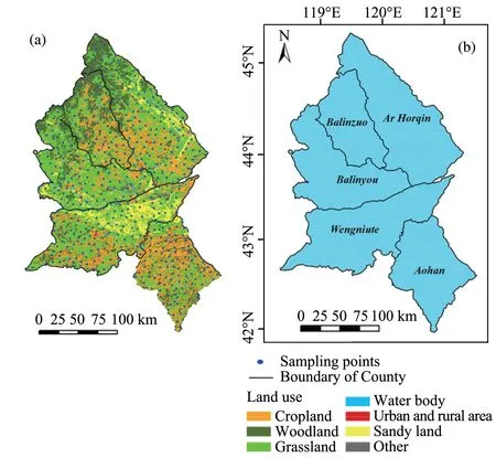
Figure 1 Locations of the study area and sampling sites.The study area is located in northeastern China,and it belongs to China's northern agro-pastoral ecotone.(a)Location of the 550 field sampling sites and land use patterns in the study area in 2015.The land use dataset was interpreted from Landsat 8 images at a scale of 1:100,000.(b)The study area includes five counties:Aohan,Wengniute,Balinyou,Balinzuo,and Ar Horqin

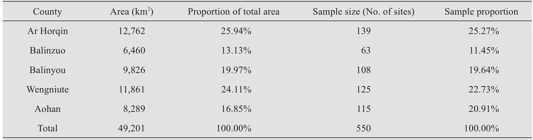
Table 1 The area of each county in the study area and the corresponding sample size

2.2 Experimental design

We obtained soil samples to a depth of 20 cm at 550 sites in the study area from April to August 2017,using a 10m×10m plot at each sampling site.We recorded the position of each sampling point with a portable GPS receiver.The samples were collected at 15 randomly selected sampling points within each plot using a soil auger (2.5 cm in diameter).The composite soil sample for each site was obtained by mixing the 15 samples evenly.We selected an additional three sampling points (replicates) in each sampling plot to determine the soil bulk density using a soil auger equipped with a stainless steel cylinder (100 cm3in volume)to obtain intact soil cores.To study the influence of different interpolation methods and random subsampling (number of sites) on the SOC estimation,we randomly selected 50 samples as the validation dataset with Subset Features tool in Geostatistical Analyst of ArcGIS 10.3 for desktop software(http://www.esri.com).The remaining 500 samples were randomly divided into groups with different sample sizes (500,400,300,200,100,and 50 samples) for use in the spatial interpolation(Figure 2).We first compared the prediction accuracy of different sample sizes with different interpolation methods, including ordinary kriging (OK), universal kriging (UK), inverse distance weighting (IDW) and radial basis function(RBF) using cross-validation, thus determining a suitable interpolation method for the present study.Furthermore, to obtain an optimal sampling density, we adopted the selected interpolation method to compare the prediction accuracy of different sample sizes by means of combining independent validation and crossvalidation.Also, since landscape heterogeneity in the study area would affect choosing the optimal sample size,we used software Fragstats 3.3 to calculate Shannon's Diversity Index (SHDI) and Shannon's Evenness Index (SHEI) in the study area, and the corresponding values were 2.01 and 0.67,respectively.

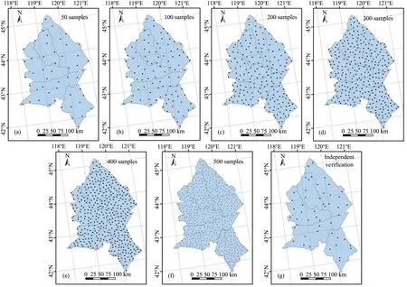
Figure 2 Locations of soil sampling sites with random subsamples ranging in size from 50 to 500 sites.A total of 50 randomly selected sites were used for independent validation of the results with these subsamples

2.3 Laboratory analyses

The collected soil samples were air-dried at room temperature, then passed through a 2 mm mesh to remove roots and other debris.We then ground a portion of each soil sample to pass through a 0.25 mmmesh before determination of the SOC concentration.It would have been prohibitively difficult to collect a full sample at a location where the sampler encountered an obstacle (e.g., a stone) larger than the sampler's diameter (2.5 cm).We therefore chose a new sampling location where we encountered coarse fragments smaller than the sampler diameter;in practice, we obtained only 30 composite samples (5.5%of the total of 550 samples) in which the coarse fragments (＞2 mm) could not be ignored.The SOC content was determined using the Walkley-Black dichromate oxidation procedure (Nelsonet al., 1996),which is widely used because it is simple and rapid and has both acceptable accuracy and minimal equipment requirements (Nelson and Sommers, 1982).A subsample of the air-dried soil was weighed and dried at 105 °C for 24 h to determine the gravimetric water content so that the SOC data could be expressed on a dry-weight basis.The bulk density(BD) was determined from soil cores obtained using a soil auger equipped with a stainless steel cylinder that was 4.2 cm in length by 5.5 cm in diameter(Blake and Hartge,1986).

2.4 SOC calculation

The SOCD (kg/m2) to a depth of 20 cm was estimated as follows:

where SOC is the SOC concentration(g/kg),BD is soil bulk density(g/cm3),D is thickness of the layer(20 cm in our study), S is the proportion of the volume occupied by coarse fragments (Cools and De Vos, 2010),and 0.01 represents a unit conversion factor.

Likewise, the SOC storage (Mt) could be estimated from SOCD and the corresponding area(km2):

2.5 Geostatistical methods

The semi-variogram is a key geostatistical function for studying soil variability.It is a continuous function that depicts the spatial autocorrelation among measured sample points.The semi-variogram is defined as follows:

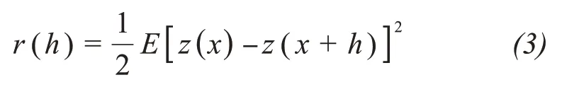
whereEis the statistical expectation, andz(x) andz(x+h) represent the paired data values being compared over a lag distance ofh(Webster and Oliver,2007).Once each pair of locations is plotted, this model can be fit through them.There are certain characteristics that are commonly used to describe these models, of which the main ones are range, sill, and nugget.A variable is considered to have a strong spatial dependence if the nugget/sill ratio is less than 25% and has a moderate spatial dependence if the ratio is between 25% and 75%; otherwise, the variable has a weak spatial dependence(Cambardella,1994).

2.6 Evaluation of prediction accuracy

We used cross-validation and independent validation to compare the performances of different predictive modeling procedures.These methods of accuracy assessment have been successfully used to compare different interpolation techniques in central Hailun County of northeastern China (Zhaoet al., 2016), the Paschim Medinipur district of India's West Bengal province (Bhuniaet al., 2016), and the Black Sea backward region of Turkey (Gölet al., 2017).For cross-validation, the trend and autocorrelation models are usually estimated by using all of the data.This approach removes each data location, one at a time, and predicts the associated data value using the remaining data (i.e., "leave-one-out validation") (Fathianet al.,2015).In a sense,cross-validation"cheats"slightly by using all of the data to estimate the trend and autocorrelation models.After completing the cross-validation, some data locations may be set aside as unusual,thereby requiring the trend and autocorrelation models to be refit.Thus, we adopted independent validation to make up for the lack of cross-validation.Independent validation first removes part of the data (the test dataset) and then uses the rest of the data (the training dataset) to develop the trend and autocorrelation models that will be used for prediction, so that the predictions can be compared with the test dataset.In our study, the test dataset comprised the 50 samples that were randomly extracted before interpolation, and the remaining 500 samples represented the training dataset for kriging interpolation.

To evaluate the predictive ability of different sample sizes with different interpolation methods, we used the mean error (ME) and the root-mean-square error(RMSE).However,the sizes of ME and RMSE depend on the sample size.Thus, we used the mean standardized error (MSE) and the root-mean-square standardized error (RMSSE) to compare the prediction accuracy with different sample sizes.The formulas for calculating these statistical indicators are as follows:

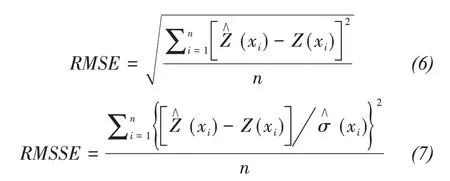
wherenrepresents the sample size,(xi) andZ(xi)represent the predicted and measured values of sampleiat locationx, respectively, and(xi) represents the standard error of the prediction.

3 Results

3.1 Descriptive statistics

Table 2 shows the descriptive statistics for the SOCD, BD, and stoniness values.The SOCD for the overall study area ranged from 0.05 to 11.24 kg/m2,with a mean of 2.24 kg/m2; the BD ranged from 0.78 to 1.63 g/cm3, with a mean of 1.31 g/cm3.From these descriptive statistics(Table 3),the coefficient of variation (CV) for SOCD for the overall study area was 66.0%,but ranged from 57.8% to 66.7%.The CV was relatively high, probably due to the high heterogeneity of the land use patterns (Figure 1c), soil types, and other factors.With increasing sample size, the minimum SOCD value decreased and the maximum value increased.In addition,the datasets for all sample sizes were not normally distributed based on the large skewness and kurtosis values.The data were therefore logarithmically converted before interpolation.The dataset with a sample size of 200 had the highest CV(66.7%), with the lowest CV (57.8%) for a sample size of 100.

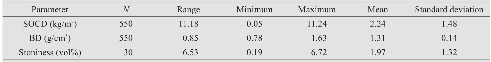
Table 2 Descriptive statistics for soil organic carbon density(SOCD),bulk density(BD)and stoniness.N represents the sample size

Table 3 Descriptive statistics for soil organic carbon density(SOCD)to a depth of 20 cm under different sampling sizes.CV,coefficient of variation

Quantitative expression and analysis of the spatial variability of soil properties are the bases for using geostatistics to predict the spatial distribution of SOCD in a study area.When the number of samples changes, the amount of information carried by the sample changes simultaneously.Table 4 shows the semi-variogram parameters for the SOCD model for each sample size.The best-fit models were all exponential.When the sample size is less than 300, the SOCD of 0-10 cm showed stronger spatial dependence than that of 10-20 cm.Especially in the 0-10 cm soil layer, the SOCD with sample size of 100 had a strong spatial dependence because their nugget/sill ratio were less than 25%.Moreover, in the 10-20 cm soil layer, the SOCD with sample sizes of 300, 400 and 500 showed strong spatial dependence.The maximum nugget/sill ratio (74.05%) appeared in the 10-20 cm soil layer with the sample size of 50.For SOCD in the layer of 0-20 cm, the minimum and maximum nuggets were 0.04 and 0.11 when the number of samples were 500 and 400, respectively.The nugget/sill ratio ranged from 13% for 500 samples to 38% for 100 samples, and the SOCD calculated with sample sizes of 200 and 500 had a strong spatial dependence.The SOCD with sample sizes of 50, 100,300, and 400 had moderate spatial dependence because their nugget/sill ratios was between 25% and 75%.As the number of samples increased, the range of the datasets gradually became smaller.The maximum range was 60.46 km when the sample size was 100, and the minimum range was 13.72 km when the sample size was 500.

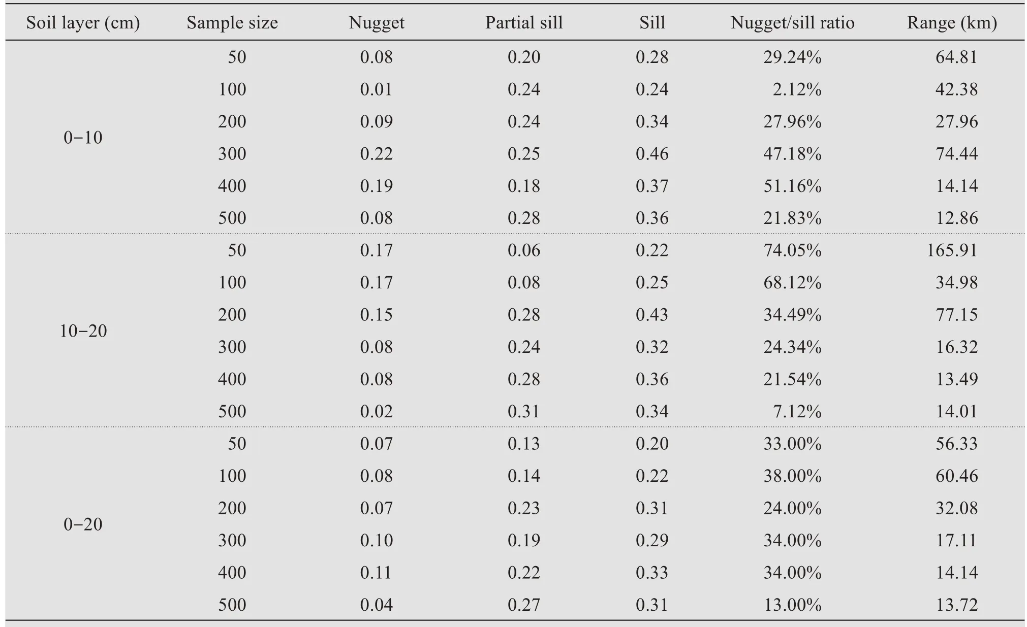
Table 4 Semi-variance parameters of soil organic carbon density(SOCD)in different soil layers under different sample sizes

3.2 Comparison of different sample sizes with different interpolation methods

We used cross-validation to calculate the ME and RMSE.Figure 3 shows the ME and RMSE values for SOCD at different sample sizes using different interpolation methods.With increasing sample size, both ME and RMSE for ordinary kriging(OK),inverse distance weighting (IDW) and radial basis function(RBF) exhibited a similar trend, where ME fluctuated around zero and RMSE ranged from 1.0 to 1.2.However, ME and RMSE under universal kriging (UK)fluctuated unstably, with an obvious peak value appeared in 300 sampling points,and its ME and RMSE were lager than corresponding values generated by the abovementioned interpolation methods.Overall,the OK method appeared to be the most accurate method, which had the smallest RMSE and the ME nearest to zero.On the contrary, the UK method performed poorly for the interpolation of SOC in the present study.

3.3 Comparison of efficiencies and errors of subsamples for SOC prediction

After determining the most accurate interpolation method, we compared MSE and ME of different sample sizes with the OK interpolation method.Figure 4 shows the ME and MSE values for SOCD at different sample sizes.The best model is the one that has the MSE and ME nearest to zero.With increasing sample size, both ME and MSE initially decreased, reaching a minimum at a sample size of 200, and then increased.The absolute value of ME decreased in the following order: 50 samples ＞ 100 samples ＞ 400 samples ＞ 500 samples ＞ 200 samples ＞ 300 samples.The absolute value of MSE decreased in the following order: 500 samples ＞ 50 samples ＞ 400 samples ＞300 samples ＞ 200 samples ＞ 100 samples.When the number of samples was 50, the prediction accuracy was very poor.

We used the test dataset of SOCD with 50 independent samples to generate the RMSE by means of independent validation, and generated the RMSSE by means of cross-validation (Figure 5).In general, the optimal model is the one that has the smallest RMSE and the RMSSE nearest to 1.The RMSE decreased initially with decreasing sample size, to a minimum at a sample size of 200; thereafter, it increased slightly.In contrast, RMSSE increased initially with increasing sample size, coming nearest to 1 at a sample size of 200.These results suggest that 200 was the optimal sample size, which is consistent with the ME and MSE validation results.This sample size can therefore produce the best accuracy with the smallest cost and amount of labor for our study area.

Figure 3 The mean error and root-mean-square error(RMSE)for SOC spatial distribution under different sampling sizes using different interpolation methods,including ordinary kriging(OK),universal kriging(UK),inverse distance weighting(IDW)and radial basis function(RBF).The dashed red line in(a)indicates y=0

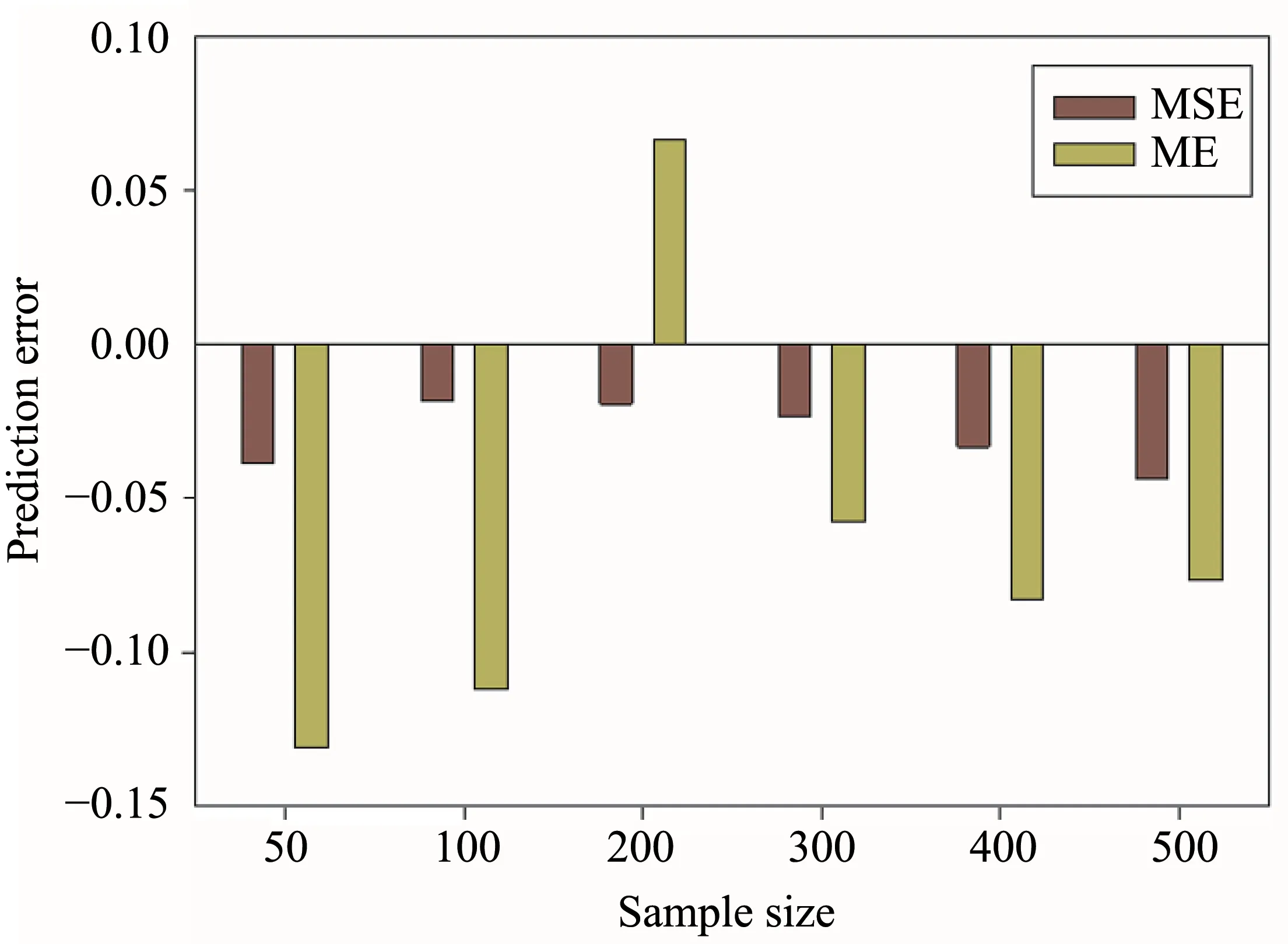
Figure 4 The mean standardized error(MSE)and mean error(ME)for SOCD in comparison with the test(validation)dataset at different sample sizes.Negative values mean that the predicted value underestimated the actual value

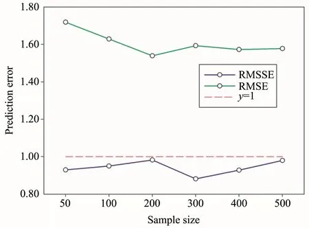
Figure 5 The root-mean-square error(RMSE)and root mean square standardized error(RMSSE)for SOCD compared with the test(validation)dataset at different sample sizes

The measured SOCD was significantly correlated with predicted value, interpolated by the OK method with different sample sizes (Figure 6).The kriging interpolated SOCD was most closely correlated with actual measurements when the sample size was 200 (R2= 0.724, slope = 0.891,P＜0.001).TheR2and slope were lowest when the sample size is less than 200 (R2= 0.409 for 50 samples and slope = 0.612 for 100 samples).These results suggest that 200 is the optimal sample size, 50 and 100 could not meet the accuracy requirements of SOCD interpolation, which is consistent with validation results.

3.4 Spatial distribution of SOCD

We used ordinary kriging interpolation to test the influence of sample size on the spatial distribution of SOCD in our study area (Figure 5).As expected, the level of detail increased with increasing sample size, allowing the interpolation to better describe the variation in SOCD.However,all five sample sizes revealed the same overall trend, with SOCD decreasing from north to south and reaching a minimum near the center-south part of the study area, and then increasing again.The sites with the highest SOCD were mainly located at the northern edge of the study area,which had the highest vegetation cover by woodland (Figure 1c).There was also a relatively high concentration located in the northern areas where there was a large area of grassland.However, SOCD was lowest in the central and southern region, which had the greatest coverage by degraded or desertified sandy land.Another area with obviously low SOCD was distributed in the southern part of the study area, where cropland accounted for a large proportion of the land cover.Thespatial distributions of SOCD were most similar when the sample size was greater than or equal to 200.This indicated that the actual spatial distribution of SOCD could still be displayed reasonably accurately using only 200 samples.In contrast, interpolation based on the two smallest sample sizes could not accurately express some details.Therefore, based on the results in Figure 7,200 sampling points appears to be a suitable choice for predicting the spatial variation of SOCD.

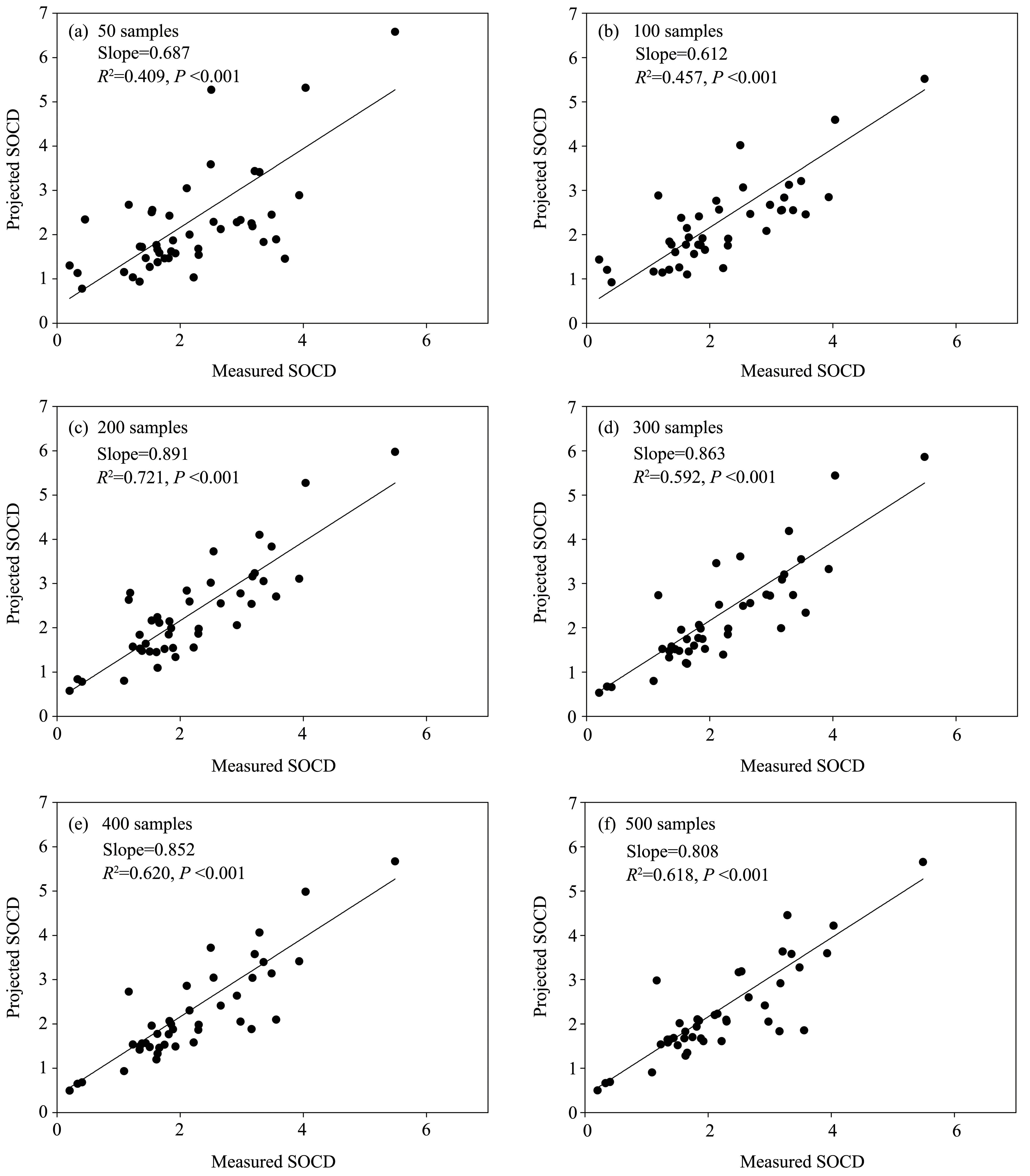
Figure 6 The relationship between measured and predicted soil organic carbon density(SOCD).The validation dataset was used to test the reliability of kriging-based SOCD estimates,which interpolated by different sample sizes(50,100,200,300,400 and 500)

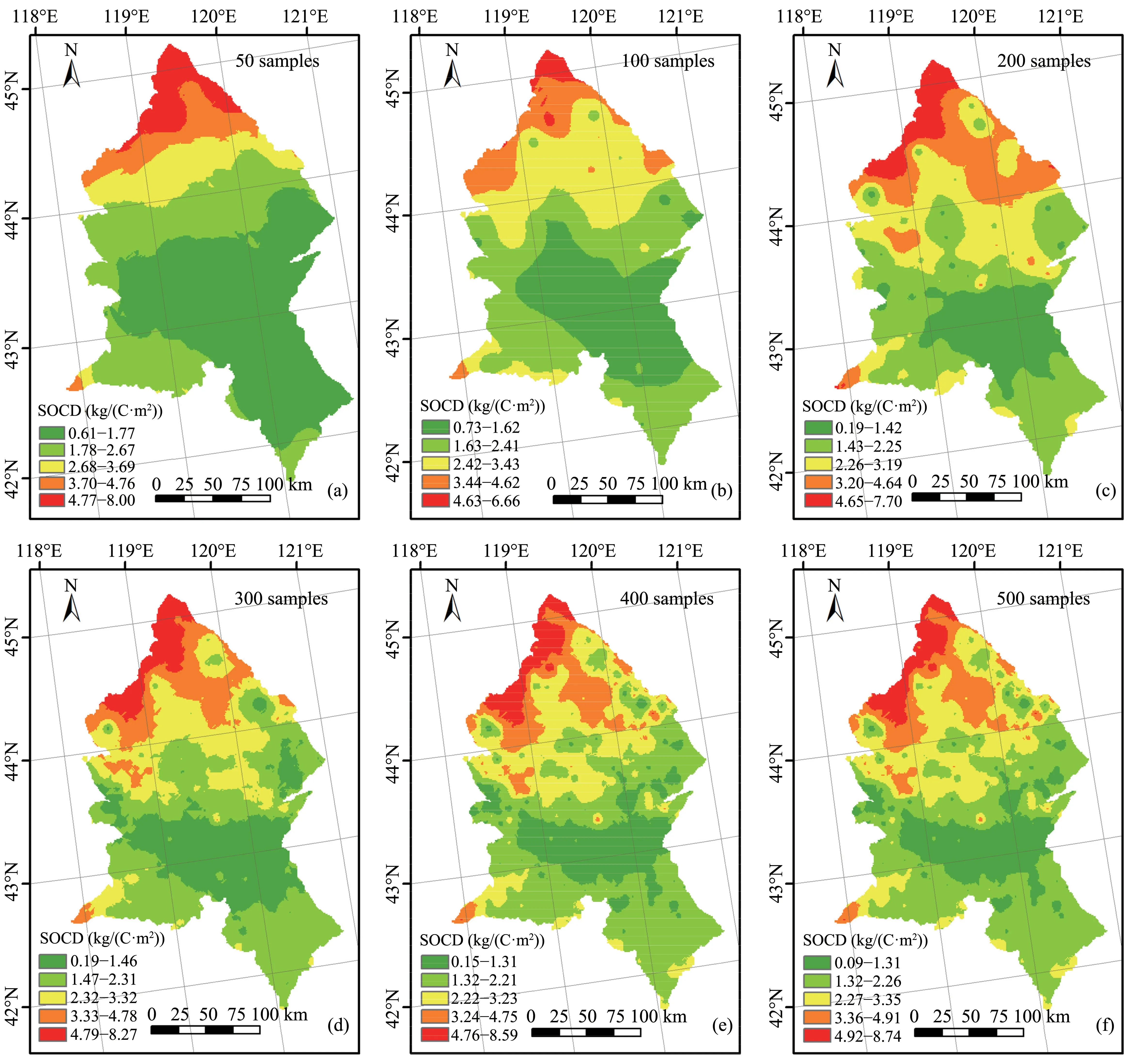
Figure 7 Spatial distribution of soil organic carbon density(SOCD)at different sample sizes using ordinary kriging interpolation

3.5 SOCD and SOC storage in different counties

Figure 8 compares mean SOCD results based on different sample sizes for each of the five counties in the study area.The SOCD changed most when the sample size was less than 300, especially in Ar Horqin and Balinzuo counties,but the SOCD tended to stabilize when the sample size was greater than or equal to 300.In Balinzuo County, the SOCD decreased strongly as the sample size increased from 50 to 100,and then increased continuously.However, we also observed increasing trends as the sample size increased from 50 to 200 in Ar Horqin and Balinyou counties.The SOCD in Balinyou was closest to the average SOCD for the entire study area.As the sample size increased, the SOCD showed little change in Wengniute and Aohan counties.Thus,changes in sample size had the greatest impact on the predicted results in Ar Horqin and Balinzuo counties.The SOCD for the total study area was relatively independent of the sample size, largely because this value represents the average for the five counties, and averaging conceals the differences among the counties.

We found that a sample size of 200 sites generated the most accurate predictions.Thus, we estimated the SOC of the five counties at this sample size based on interpolation results (Table 5).The total SOC storage in the study area was 117.94 Mt,and itsmean SOCD was 2.40 kg/m2.The mean SOCD (kg/m2)was ranked in the following order: Balinzuo (3.29±1.32) ＞ Ar Horqin (3.21±1.04) ＞ Balinyou (2.41±0.91) ＞ Aohan (1.61±0.41) ＞ Wengniute (1.57±0.73).However, the largest storage was 41.02 Mt in Ar Horqin County, and the lowest storage was 13.35 Mt in Aohan.This resulted from the different areas of the counties.

Figure 8 The mean soil organic carbon density(SOCD)to a depth of 20 cm at different sample sizes for the five counties in the study area and for the study area as a whole

Table 5 The soil organic carbon density(SOCD)and storage to a depth of 20 cm for the five counties in the study area.Min and Max represent minimum and maximum densities,and SD is the Standard Deviation

4 Discussion

4.1 The spatial dependence for different sample sizes

In general, a variable is considered to have a strong spatial dependence if the nugget/sill ratio is less than 25% and moderate spatial dependence if the ratio is between 25% and 75%; otherwise, the variable has a weak spatial dependence (Cambardella, 1994).In our research, the nugget/sill ratio ranged from 13% to 38% (Table 4), and the SOCD with both 200 and 500 samples exhibited a strong spatial dependence, with nugget/sill ratios of 24% and 13%,respectively.The SOCD based on sample sizes of 50, 100, 300, and 400 had moderate spatial dependence, with a nugget/sill ratio that ranged from 33%to 38%.These nugget/sill ratios were close to those for SOC in the state of Pennsylvania, United States(38%)(Kumaret al.,2012),Changbai Mountain Natural Reserve in northeastern China (23.8%) (Yuanet al., 2013), and Beichuan County in northwestern China (28.8%) (Maiet al., 2105).However, the nugget/sill ratio was much higher than the value (0.2%)in a small watershed in a hilly area of Northern China (Gaoet al., 2013).Differences in the sample size,geomorphology, topography, vegetation cover, land use, and climate can likely explain these differences(Yanget al.,2013).

4.2 The effects of interpolation methods and sample size on accuracy of SOCD estimates

Many studies have shown that the OK method has better prediction accuracy for SOCD estimates than other interpolation methods (Zareet al.,2011;Yasrebiet al., 2012; Bhuniaet al., 2016; Zhaoet al., 2016),which is consistent with our results.However, in a representative county of the hilly Red soil region in southern China,Zhanget al.(2015)applied two interpolation methods of ordinary kriging (OK) and kriging combined with land use information(LUK)to predict spatial distribution of SOCD,and the results demonstrated that the OK method is not very suitable to predict SOC spatial variability.The interpolation method is sensitive to the prediction accuracy of SOCD estimates, and efficient interpolation method would contribute to obtain high-precision SOC distribution information.

The prediction accuracies varied greatly among sampling densities, and the effects of sample size differed among the regions.In some regions, the SOCD prediction error decreased with increasing sampling density (Heimet al., 2009; Steffenset al., 2009),whereas the prediction accuracy was not improved in other regions (Liet al., 2007; Sahrawatet al., 2008;Sunet al., 2012).It is generally believed that prediction accuracy will be more sensitive to sampling density in areas of complex terrain than in areas with simple terrain (Yuet al., 2011).Figure 9 shows that our study area has complex terrain, with an elevation that ranged from 257 m to 1,958 m, with the elevation gradually increasing from east to west.This topographic variation explains why the prediction accuracy of SOCD differs greatly between counties in response to changes in sample density.

The RMSE for SOCD was lowest with 200 samples(1.54 kg/m2)using ordinary kriging,with a similarly small ME (0.07 kg/m2),but the ME was smallest with 300 samples (-0.06 kg/m2).Both RMSE and ME were smaller than the prediction errors produced by means of a geographically weighted regression approach (RMSE = 6.40 kg/m2and ME =-0.11 kg/m2) (Mishraet al., 2010), and they were also lower than previous prediction errors (RMSE =2.68 g/kg and ME = -0.11 g/kg) when the sampling density was 1 sample per 8 km2and interpolation used ordinary kriging (Sunet al., 2012).In addition, the RMSE of SOCD generated by means of ordinary kriging (0.11%) was smaller than values obtained in previous research using other interpolation methods, including a radial basis function, inverse distance weighting, local polynomial interpolation, and empirical Bayesian kriging (Bhuniaet al.,2016).

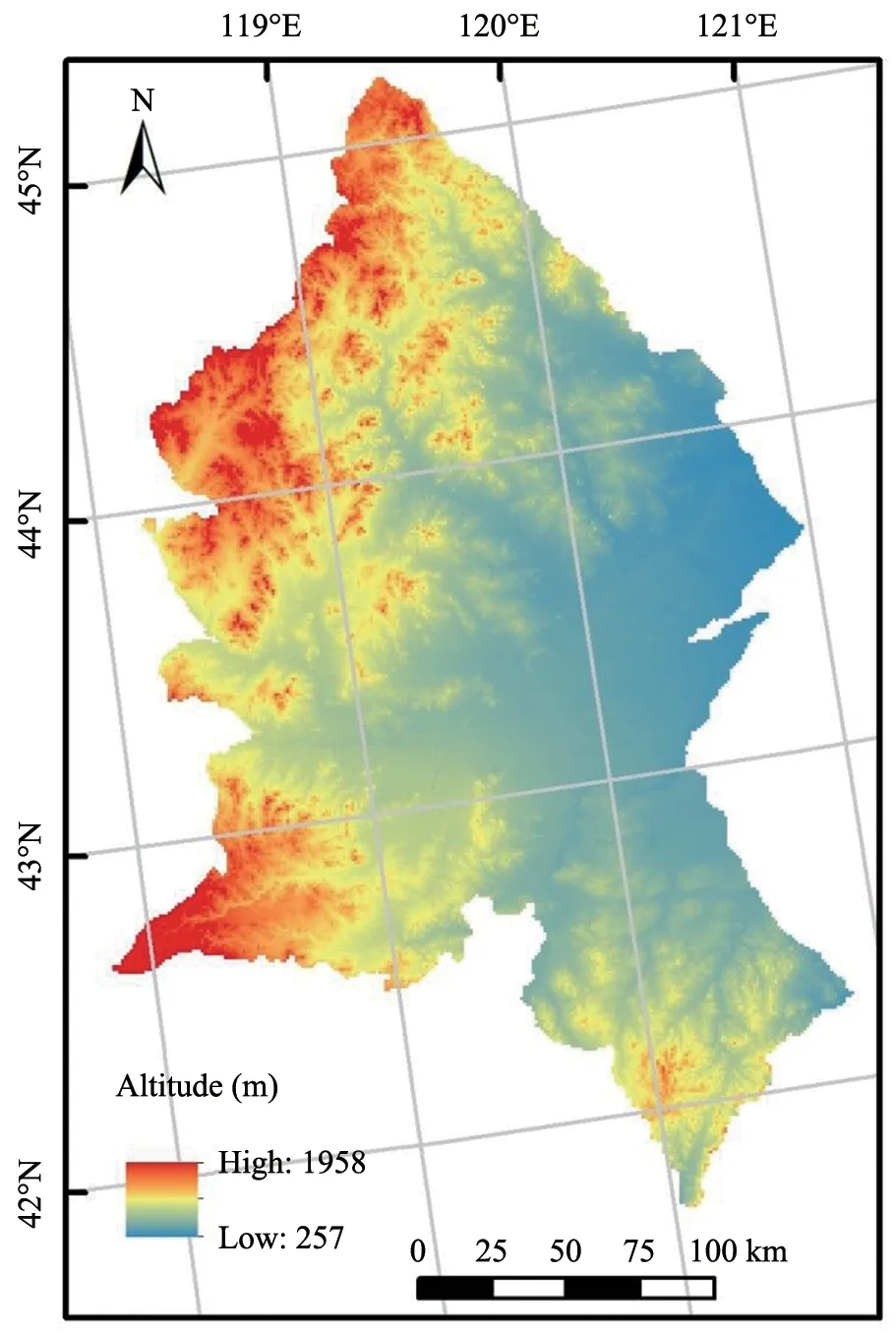
Figure 9 Topography(elevation)of the study area in Northern China

When predicting SOCD and heavy metal contents,the prediction accuracy tends to decrease as the sample size decreases(Liuet al.,2006;Simbahan and Dobermann, 2006; Chenet al., 2009).Overall, our results confirmed this trend, but with a difference: the prediction accuracy was highest with 200 sampling points, and decreased thereafter.Although we did not account for sampling costs in our analysis, a sampling scheme based on this sample size may represent a good balance between accuracy and the sampling cost and effort.Previous results by Boivin and Gascuel-Odoux(1994)agreed with our results.Other researchers found that the RMSE of the predicted SOCD stock to a depth of 30 cm decreased with sample size increasing from 50 to 200 for ordinary kriging(Simbahan and Dobermann, 2006).This is also consistent with the trend for SOCD to a depth of 20 cm in the present study.

The predicted SOCD changed most when the sample size increased from 50 to 300,but the SOCD tended to remain stable when the sample size was greater than or equal to 300.Hence,changes in the interpolated SOCD are more sensitive to datasets with a smaller number of samples.Therefore, when using ordinary kriging for SOCD prediction, we predict that SOCD will change most at small sample sizes, and that SOCD will stabilize when the number of sampling points is large enough.However, additional field research will be required to confirm this hypothesis.

4.3 The effects of sample size on spatial distri‐bution of SOCD

In terms of the spatial distribution of SOCD, the ability to reveal details generally decreases with decreasing sampling density (Liaoet al., 2009; Zhanget al., 2015).Our results confirm this: the sample with 500 points provided the most detailed expression of the spatial distribution of SOCD, whereas sample sizes of 50 and 100 did not accurately reflect the distribution of SOCD.However,200 sampling points presented a satisfactory expression of the spatial distribution of SOCD.Thus, this sample size may be adequate in future research in the agro-pastoral ecotone of northern China if the research is supported by providing sufficient funding.

4.4 The effects of land use and cover on SOCD in different counties

Though climate is one of the major factors that affect SOCD,we ignored climatic factors in the present study because all five counties in the study area had a similar continental semi-arid monsoonal climate (Liet al., 2004).Land use and cover type is widely considered to affect SOC (Wilsonet al., 2011;Wiesmeieret al., 2012).Table 6 summarizes the proportions of the total area in each land use and cover type category in the five counties.Balinzuo had the largest woodland proportion (36.2%), whereas the sandy area was largest in Wengniute County, accounting for 19.7% of the county area, the SOCD of woodland in Balinzuo was 3.93 kg/m2, and the SOCD of sandy area Wengniute County was 0.86 kg/m2(Table 7).These differences of land use proportion explain why Balinzuo and Wengniute had the highest and lowest SOCD, its corresponding values was 3.29 kg/m2and 1.57 kg/m2, respectively (Table 5).For total study area in the present study,the SOCD (kg/(C·m2))to a depth of 20 cm was in the following order:woodland(3.29)＞grassland(2.35)＞cropland(2.19)＞sandy land (1.55) (Table 7), woodland and grassland tend to store more SOC than cropland due to the large amounts of aboveground biomass and abundant roots in woodland and grassland, which promote accumulation of soil organic matter (Xue and Zhang,2013).For cropland, the relatively low SOCD was mainly due to the removal of plant residues during harvesting, which could significantly reduce the input of organic matter (Wiesmeieret al., 2013).The severe wind erosion removed amounts of organic matter input, which is in the form of litter and fine particles, leading to the lowest SOCD in sandy land(Li and Shao,2014).

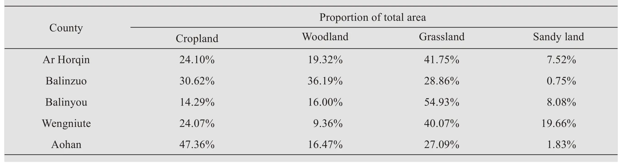
Table 6 The proportions of the main land use and cover types in each county

5 Conclusions

Our study area includes a wide variety of landscape types (SHDI = 2.01 and SHEI = 0.67), and our results suggest that the ordinary kriging approach is a promising method for regional-scale prediction of SOCD.In addition, the accuracy of SOCD prediction was greatly influenced by the sample size in our study area in the agro-pastoral ecotone of northern China.The results of cross-validation and independent validation shows that the sampling size of 200 provided the most accurate prediction of SOCD, with RMSE =1.54 kg/m2and ME = 0.07 kg/m2, whereas the smallest sample size (50) provided the worst prediction accuracy.Based on the size of our study area, the optimal average sampling density of 200 points is the equivalent of 0.004 points per km2(about 1 point per246 km2).In terms of the spatial distribution of SOCD, the ability to reveal detailed patterns increases with increasing sample size, but the sample size of 200 appears to represent an acceptable compromise between sampling resolution and cost (money and labor).

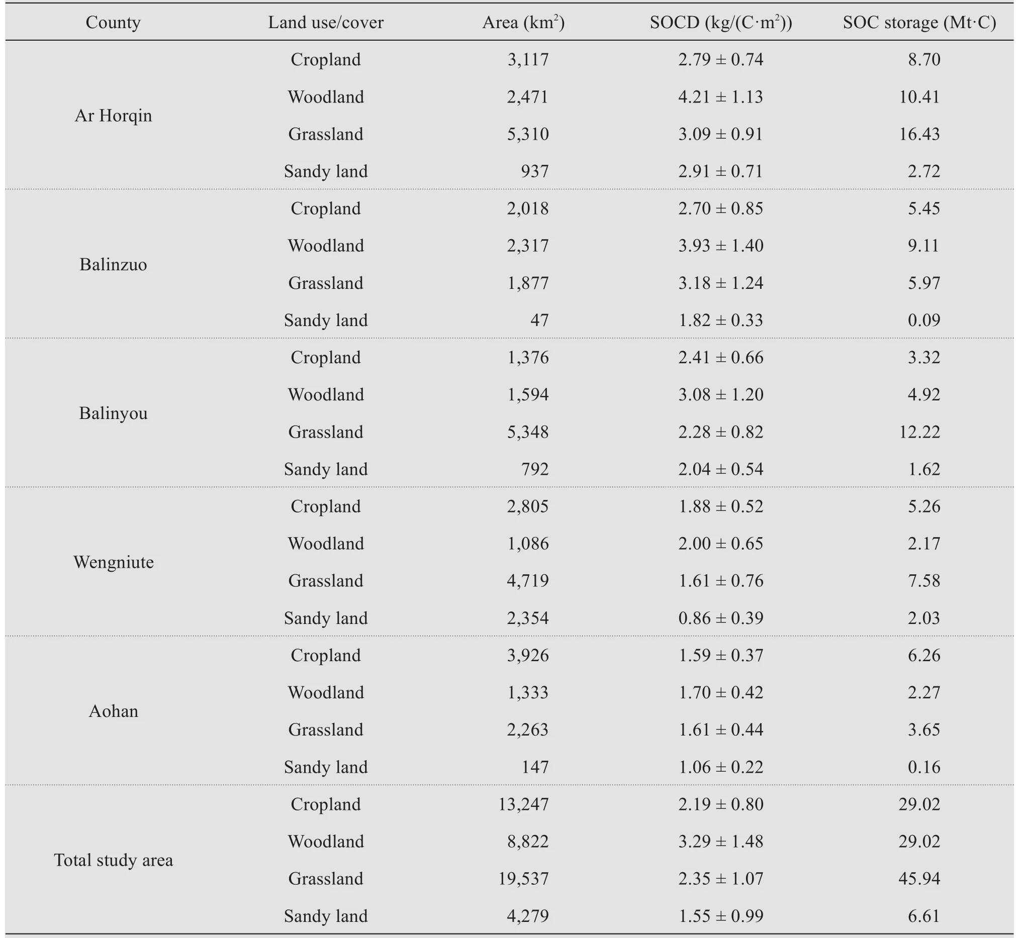
Table 7 The soil organic carbon density(SOCD)and storage to a depth of 20 cm among different land use types for each county and total study area

The predicted SOCD varied drastically among sample sizes, but tended to stabilize when the sample size was greater than or equal to 300.The mean SOCD varied among the counties in response to differences in their topography and their land use and cover types.

Acknowledgments:

This research was supported by the National Key R and D Program of China (2016YFC0500901 and 2016YFC0500907), the National Natural Science Foundation of China (Grant Nos.31971466 and 41807525), and the One Hundred Person Project of the Chinese Academy of Sciences(Y551821).