Long Time Well-Posedness of the MHD Boundary Layer Equation in Sobolev Space

Dongxiang Chen,Siqi Ren,Yuxi Wang and Zhifei Zhang,*

1 College of Mathematics and Information Science,Jiangxi Normal University,Nanchang,Jiangxi 330022,China

2 Department of Applied Mathematics,Zhejiang University of Technology,Hangzhou,Zhejiang 310032,China

3 School of Mathematical Sciences,Peking University,Beijing 100871,China

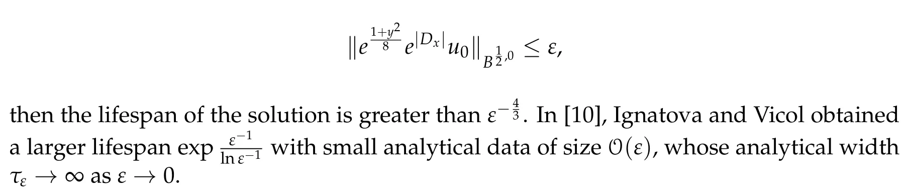
Abstract. In this paper,we study the long time well-posedness of 2-D MHD boundary layer equation. It was proved that if the initial data satisfies

Key Words: MHD boundary layer equation,Sobolev space,well-posedness.

1 Introduction

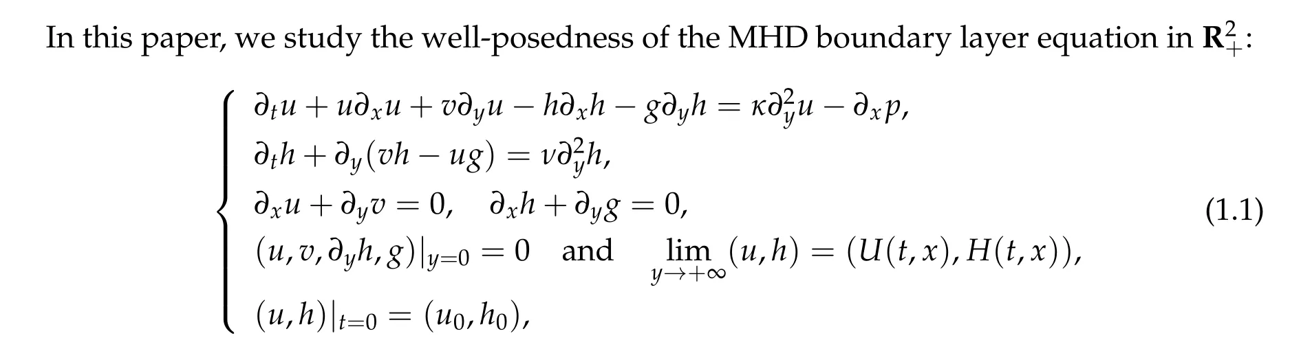
where(u,v)denotes the velocity field of the boundary layer flow,(h,g)denotes the magnetic field, and (U(t,x),H(t,x),p(t,x)) denotes the outflow of velocity, magnetic and pressure,which satisfies the Bernoulli’s law:

This system is a boundary layer model,which describes the behaviour of the solution of the viscous MHD equations when the viscosity and the resistivity tend to zero[6,11].When h=0,the system(1.1)is reduced to the classical Prandtl equation:

The well-posedness theory of the 2-D Prandtl equation was well understood. For the monotonic data, Oleinik [14] proved the local existence and uniqueness of classical solutions. With the additional favorable pressure, Xin and Zhang [16] proved the global existence of weak solutions of the Prandtl equation. Sammartino and Calflisch [15] established the local well-posedness of the Prandtl equation for the analytic data. Recently, Alexandre et al. [1] and Masmoudi-Wong [13] independently developed direct energy method to prove the well-posedness of the Prandtl equation for monotonic data in Sobolev spaces. Without monotonicity, G´erard-Varet and Dormy [7] proved the illposedness of the Prandtl equation in Sobolev space. However, the Prandtl equation is well-posed in Gevrey class 2 for a class of non-monotone data with non-degenerate critical points[4,8,12].On the other hand,E and Engquist[5]proved that the analytic solution can blow up in a finite time[5]. See[9]for the extension to van Dommelen-Shen type singularity. For small analytic initial data,Zhang and the fourth author[18]proved the long time well-posedness of the Prandtl equation: if the initial data satisfies

In two recent interesting works [6,11], the authors showed that the tangential magnetic field has stabilization effect on the boundary layer of the fluid. In particular, they proved the well-posedness of the system (1.1) for the data without monotonicity under an uniform tangential magnetic field.

The goal of this paper is two folds:(1)present a simple proof of well-posedness based on the paralinearization method developed in[3];(2)study the long time well-posedness of the system (1.1) for small data in Sobolev space. In [17], Xu and Zhang proved a long time existence of the Prandtl equation for the data close a monotonic shear flow.However, it is unclear how the lifespan of the solution depends on the data. Here we would like to give the explicit lifespan of the solution of the system(1.1).

For simplicity,we consider a uniform outflow(U,H)=(0,1)and take κ = ν=1. Let

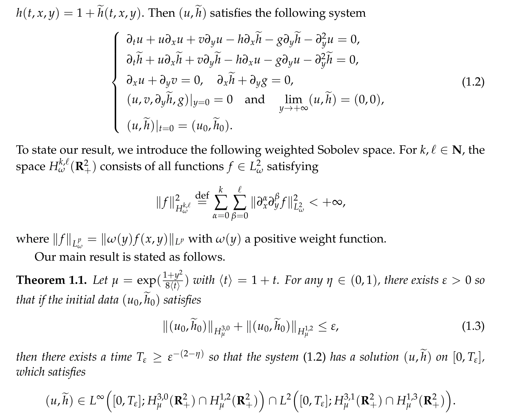
Remark 1.1. It is unclear whether the lifespan of the solution obtained in Theorem 1.1 is sharp. It remains open whether the solution is global in time for small data.

2 Littlewood-Paley decomposition and paraproduct

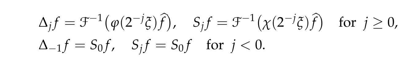
We first introduce the Littlewood-Paley decomposition in the horizontal direction x ∈R.Choose two smooth functions χ(τ)and φ(τ),which satisfy

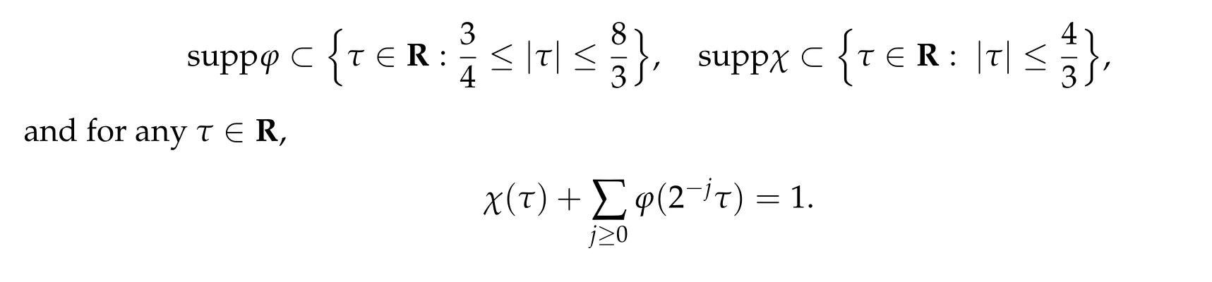
Then we define

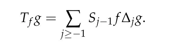
The Bony’s paraproduct Tfg is defined by

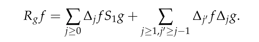
Then we have the following Bony’s decomposition

where the remainder term Rgf is defined by

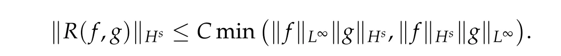
We denote by Ws,pthe usual Sobolev spaces in R and denote Ws,2by Hs. Let us recall classical paraproduct estimates and paraproduct calculus.

Lemma 2.1. Let s ∈R. It holds that

If s ＞0,then we have

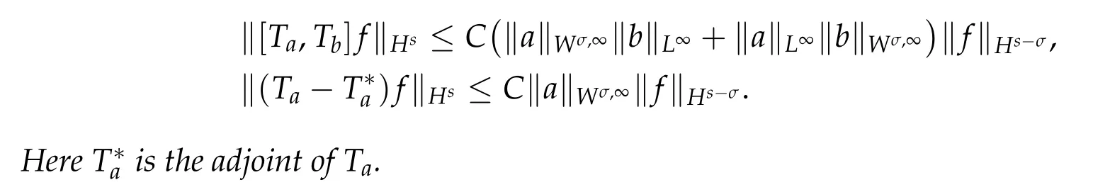
Lemma 2.2. Let s ∈R and σ ∈(0,1]. It holds that

Especially,we have

Lemma 2.3. Let s ∈N. It holds that

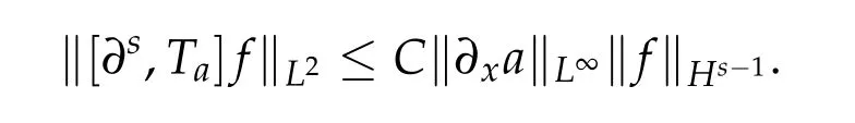
Let us refer to[2]for more introduction.

3 Paralinearization and symmetrization

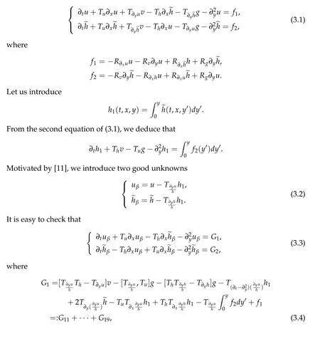
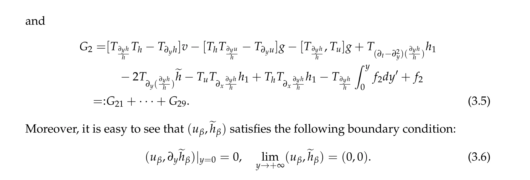
As in the Prandtl equation, an essential difficulty in solving the MHD boundary layer equation is the loss of one derivative in the horizontal direction induced by the terms like v∂yu,v∂yh,g∂yu,g∂yh. To overcome this difficulty, motivated by [3], we will first paralinearize the system (1.2), and then introduce good unknowns to symmetrize the system following the idea in[11].

Using Bony’s decomposition(2.1),we can rewrite the system(1.2)as

4 Sobolev estimate in horizontal direction

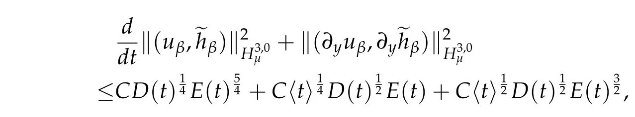
Proposition 4.1. It holds that for any t ∈[0,T],

4.1 Some technical lemmas

Lemma 4.1. There exists ε0＞0 so that if ε ∈(0,ε0),then

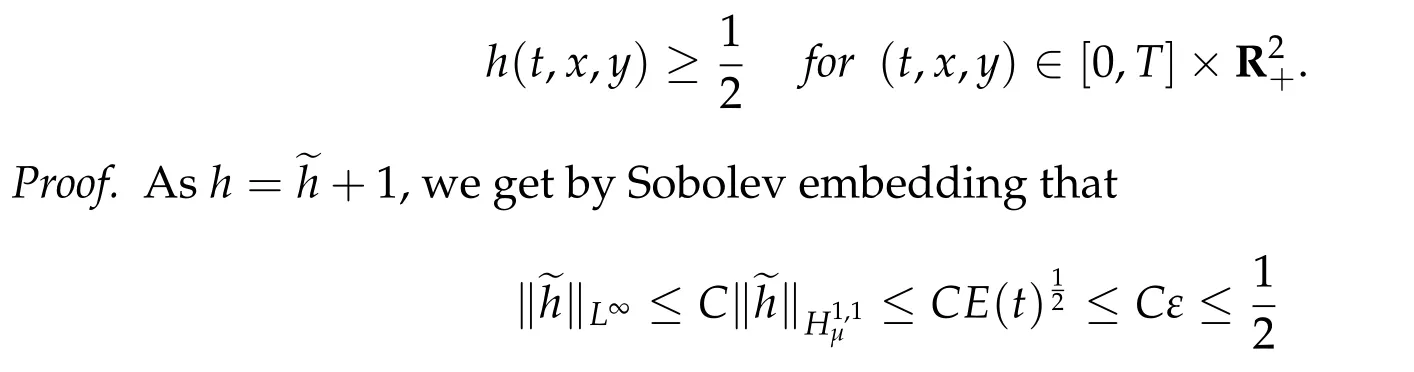
by taking ε0small enough.

The following lemma is a direct consequence of H¨older inequality.

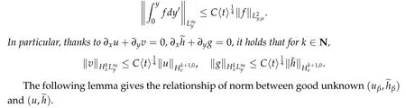
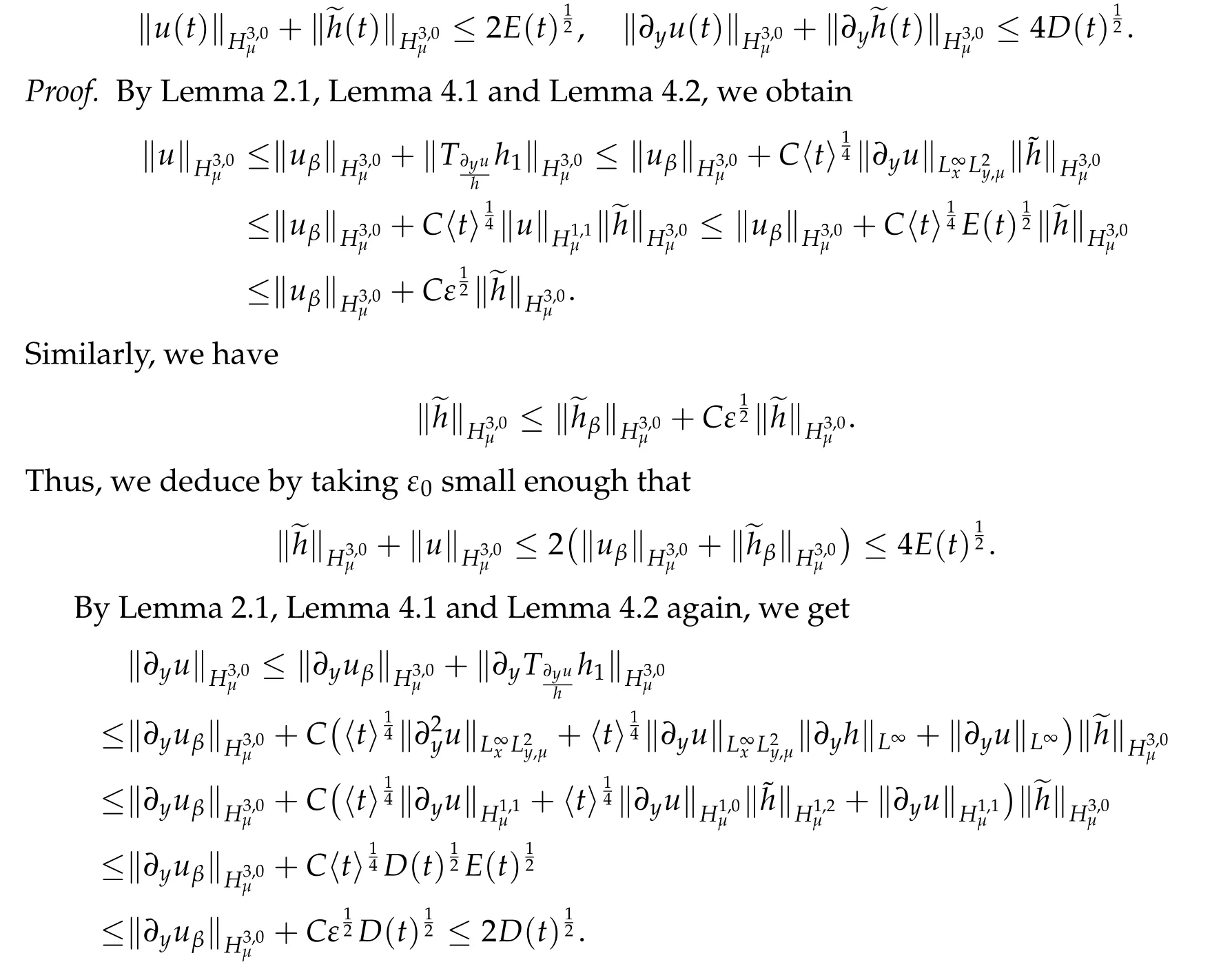
Lemma 4.2. It holds that

Lemma 4.3. There exists ε0＞0 so that if ε ∈(0,ε0),then for t ∈[0,T],

In the same way,we have

This proves the lemma.

4.2 Nonlinear estimates

Let us now estimate the nonlinear terms G1and G2.

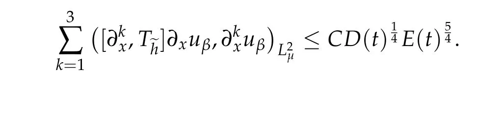
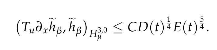
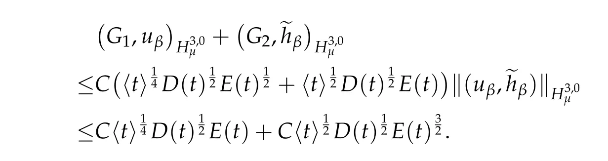
Lemma 4.4. It holds that

Proof. Let us only present the estimate of G1. The estimate of G2is similar. By Lemma 2.2,Lemma 4.1 and Lemma 4.2,we have

Using the facts that

we can deduce from Lemmas 2.2,4.1 and 4.2 that

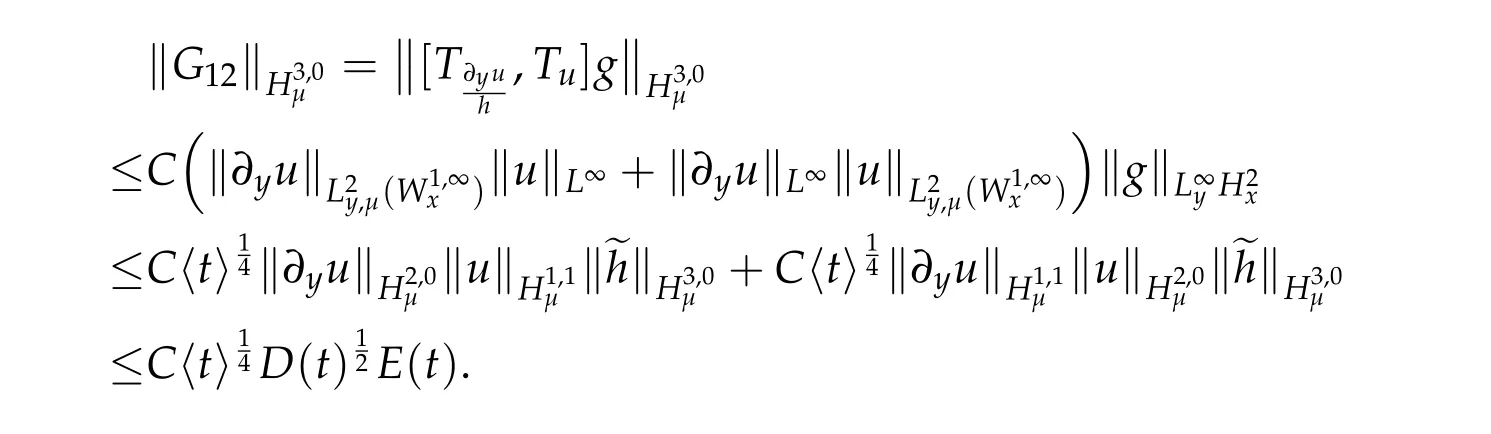
Similarly,we have

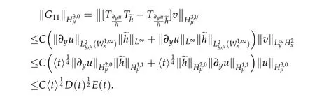
Thanks to Lemma 2.1 and Lemma 4.1,we have

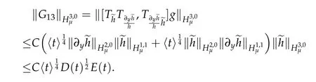
By Lemma 2.1,Lemma 4.1 and Lemma 4.2,we get

Similarly,we have

For G14,we use Eq.(1.2)to find that

Using Lemmas 2.1,4.1 and 4.2,we deduce that

Thus,we conclude that

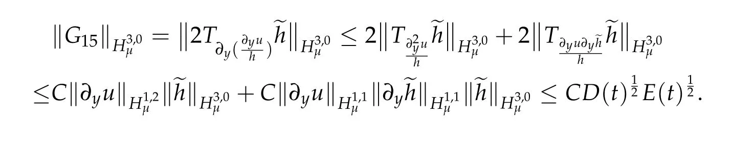
Using

and Lemma 2.1,we have

which gives

Similarly,we have

Putting all the above estimates together leads to the estimate of‖G1‖H3,0μ.

4.3 Tangential energy estimate

In this subsection,we prove Proposition 4.1.

First of all,we have

we get by integration by parts that

Similarly,we have

We write

where

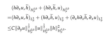
By Lemma 2.1 and Lemma 2.2,we have

and by Lemma 2.3,

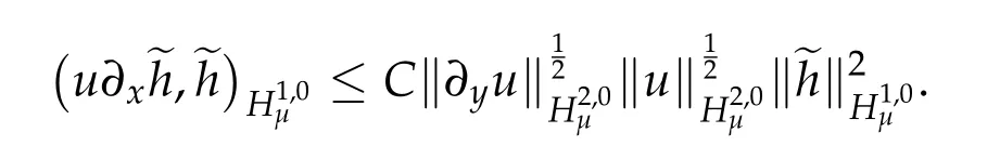
This shows that

Similarly,we have

On the other hand,we write

Thus,we also have

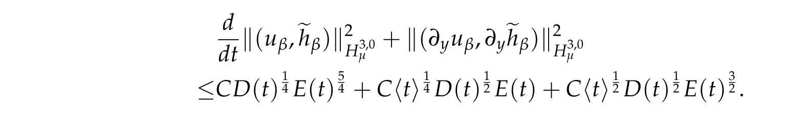
It follows from Lemma 4.4 that

Summing up all the estimates,we conclude that

where we used ∂tθ+2(∂yθ)2＜0.

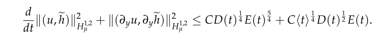
5 Sobolev estimate in vertical direction

Proposition 5.1. It holds that for any t ∈[0,T],

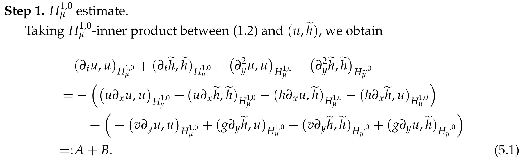
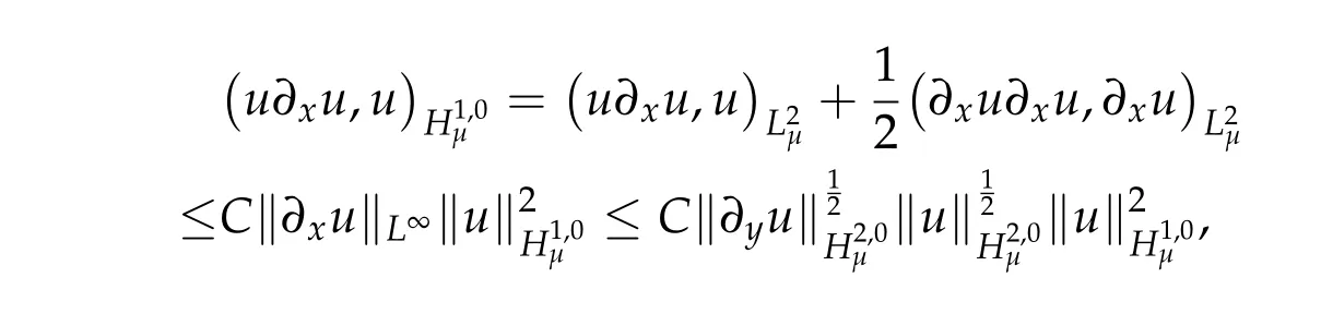
Proof. We split the proof into the following three steps.

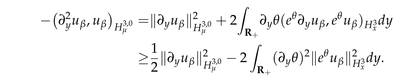
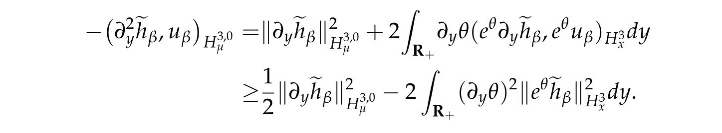
By integrating by parts and thanks to ∂tθ+2(∂yθ)2≤0,we have

By integration by parts,we get

and

Similarly,we have

This shows that

The other terms in B could be estimated in a similar way. Then we have

Thus,we deduce that

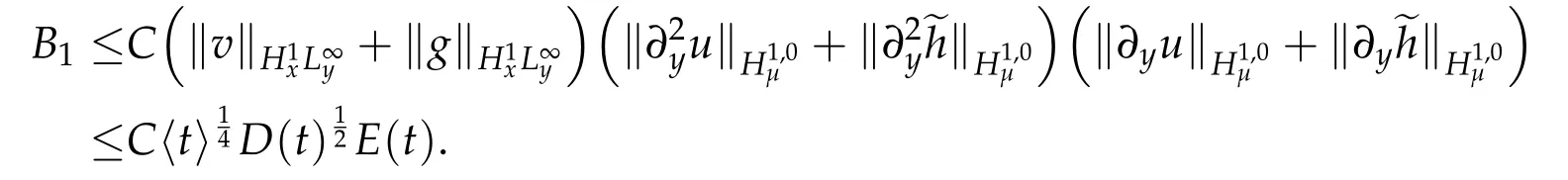
and for B1,we have

and for C1,we have

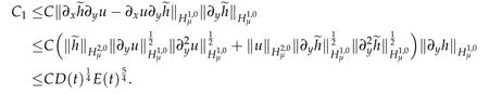
Thus,we deduce that

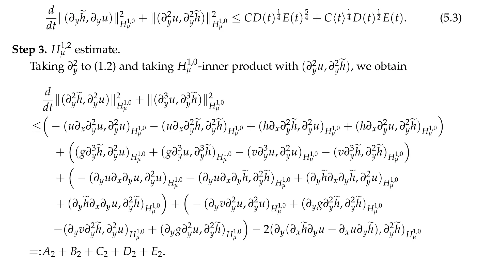
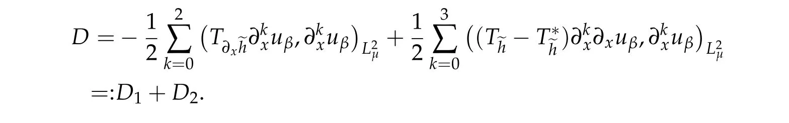
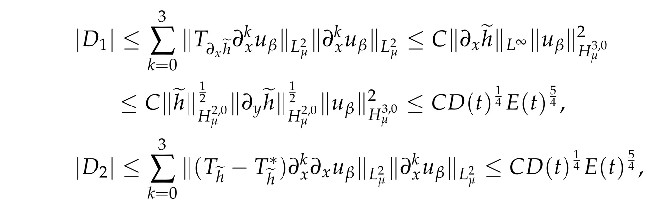
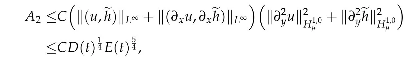
We estimate nonlinear terms as follows:

and

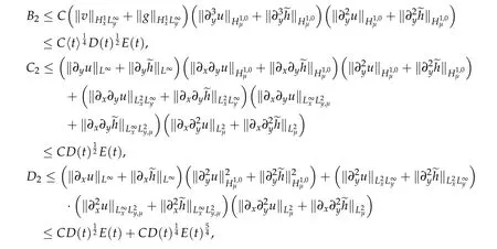
and

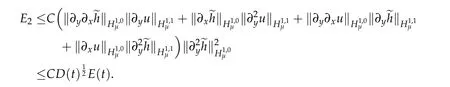
This shows that

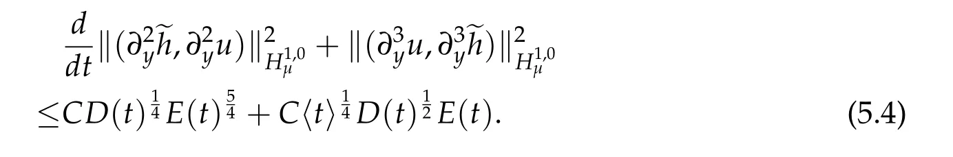
Then the proposition follows from(5.2)-(5.4).

6 Proof of Theorem 1.1

We first introduce the following Poincar´e type inequality.

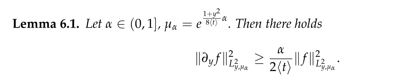
Proof. A direct calculation gives

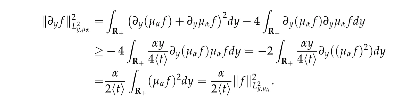
Thus,we complete the proof.

Now we prove Theorem 1.1.

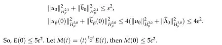
Thanks to the initial condition and Lemma 4.3,we have

The uniform estimate is based on a bootstrap argument. Let us first assume that[0,T*)is the maximal time interval so that

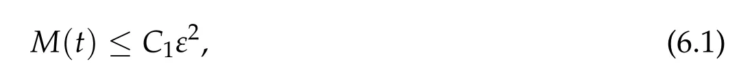
where C1＞0 is a fixed constant. Let us also assume T*＜ε-2.

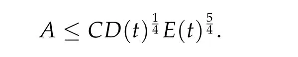
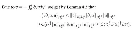
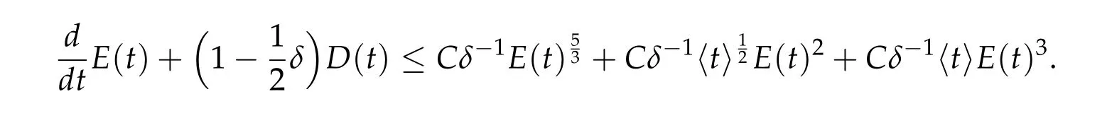
Thanks to E(t)≤C1ε2,it follows from Proposition 4.1 and Proposition 5.1 that

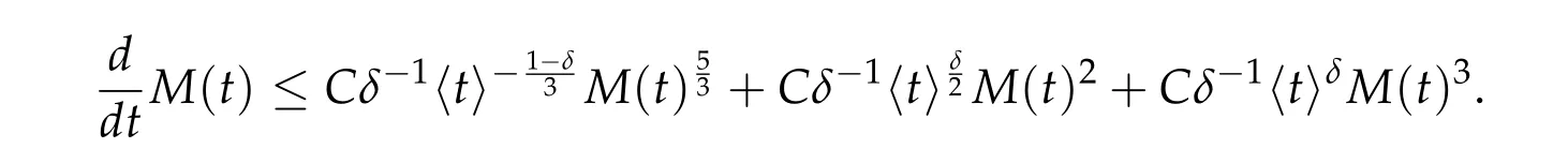
Let δ ∈(0,1)be determined later. Then we have

Thanks to Lemma 6.1 with α=1,we get

which gives

Thus,for given η ∈(0,1),there exists δ ＞0 so that for t ≤ε-2+η,

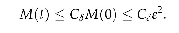
Taking C1=2Cδ,the theorem follows by a bootstrap argument.

Acknowledgements

Z.Zhang is partially supported by NSF of China under Grant No.11425103.