CONVERGENCE OF CONTROLLED MODELS FOR CONTINUOUS-TIME MARKOV DECISION PROCESSES WITH CONSTRAINED AVERAGE CRITERIA∗†

Wenzhao Zhang, Xianzhu Xiong

(College of Math.and Computer Science,Fuzhou University,Fuzhou 350108,Fujian,PR China)

Abstract This paper attempts to study the convergence of optimal values and optimal policies of continuous-time Markov decision processes(CTMDP for short)under the constrained average criteria. For a given original model M∞of CTMDP with denumerable states and a sequence{Mn}of CTMDP with finite states,we give a new convergence condition to ensure that the optimal values and optimal policies of{Mn}converge to the optimal value and optimal policy of M∞as the state space Sn of Mn converges to the state space S∞of M∞,respectively.The transition rates and cost/reward functions of M∞are allowed to be unbounded.Our approach can be viewed as a combination method of linear program and Lagrange multipliers.

Keywords continuous-time Markov decision processes;optimal value;optimal policies;constrained average criteria;occupation measures

1 Introduction

Markov decision processes have wide application in queueing system,telecommunications systems,etc.;see,for instance,[2,11,13,16,18]and the reference therein.The existence and computation of optimal value and optimal policies form a hot research area in Markov decision processes.The basic method to study the existence of optimal policies include the dynamic programming approach,the linear programming and duality programming method.Based on above methods,the value iteration algorithms,policy iteration algorithms,linear programming algorithms for unconstrained optimality problems and linear programming algorithms for constrained optimality problems have been proposed; see,for instance,[4,11,13,15]. However,these algorithms are only adapt to tackle the optimality problems with finite states.It is natural to use finite-state models to approximate the original model with denumerable state space or general Borel state space.Hence,from the theoretical and practical point of view,the convergence of optimal values and optimal policies are important and interesting issues in Markov decision processes.

In the discrete-time context,[3]considered the convergence of optimal value and optimal policies of Markov decision processes with denumerable states under the constrained expected discounted cost criteria.[5,6]developed the approximation method of optimal value and optimal policies of Markov decision processes with Borel state and action spaces under the constrained expected discounted cost criteria.

In the continuous-time formulation,[16]studied the convergence of optimal value and optimal policies of Markov decision processes with denumerable states under the expected discounted cost and average cost criteria.[17,18]developed an approximation procedure for CTMDP with denumerable state space under the finitehorizon expected total cost criterion and risk-sensitive finite-horizon cost criterion,respectively.For constrained optimal problem,[12]proposed an approach based on occupation measures to study the convergence problem of optimal value and optimal policies,and gave condition imposed on the original model with denumerable states to ensure the original model can be approximated by a sequence of CTMDP with finite states.

In this paper,we consider the similar convergence problem as in[12]with denumerable states but under the constrained expected average criteria.More precisely,the original controlled model has the following features:1)The state space is denumerable and the action space is a Polish space;2)the transition rates,cost and reward functions may be unbounded from above and from below.Firstly,by introducing the average occupation measures and Lagrange multipliers,we prove that the constrained optimality problem of each model Mnof CTMDP equals to a unconstrained optimality problem,and deduce the optimality equation which includes some Lagrange multipliers. These results are extension of the results in[16]for constrained optimality problem with one constraint.Then,we derive the bound of the Lagrange multipliers in each model Mn.Secondly,according to the optimality equations,we give the exact bound of of the optimal values between the finite-state model Mnand the original model M∞.Finally,using some approximation properties of expected average reward/cost,we obtain the asymptotic convergence of optimal policies of finite-state models to the optimal policy of the original model.

The rest of the paper is organized as follows. In Section 2,we introduce the constrained average model we are concerned with. In Section 3,we deduce the optimality equation of each constrained model Mnand give the error bounds of the Lagrange multipliers in optimality equations.In Section 4,we obtain the asymptotic convergence of optimal values of finite-state models to the optimal value of the original model and asymptotic convergence of policies of finite-state models to the optimal policy of the original model.

2 The Models

In this section we introduce the models we are concerned with.

NotationIf X is a Polish space,we denote by B(X)its Borel σ-algebra,by P(X)the set of probability measures on B(X)endowed with the topology of weak convergence,bythe Banach space of all bounded measurable functions on X,bythe Banach space of all bounded continuous functions on X. Letand

Consider the sequence of models{Mn}for constrained CTMDP:

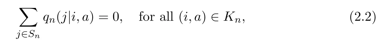
where Snis the state space. We assume Sn:={0,1,···,n}for eachand S∞:={0,1,···}.As a consequence,for each i ∈S∞,we can define n(i):=min{n ≥1,i ∈Sn}.The set A is the action space which is assumed to be a Polish space and the set A(i)∈B(A)represents the set of all available actions or decisions at state i ∈Snfor eachLetrepresent the set of all feasible state-action pairs.For fixedthe function qn(·|i,a)in(2.1)denotes the transition rates,that is,qn(j|i,a)≥0 for all(i,a)∈Knand ij.Furthermore,qn(i|j,a)is assumed to be conservative,that is

and stable,that is

Moreover,qn(j|i,a)is a measurable function on A(i)for each fixed i,j ∈Sn.Finally,rncorresponds to the reward function that is to be maximized,andcorresponds to the cost function on which the constraintis imposed for each 1 ≤l ≤p.The γndenotes the initial distribution for Mn.

Next,we briefly recall the construction of the stochastic basis(Ωn,Fn,{Ft,n}t≥0,for each n ∈N. Let i∞S∞be an isolated point andThus,we obtain the sample space(Ωn,Fn),where Fnis the standard Borel σ-algebra.For each m ≥1 and each sample ω=(i0,θ1,i1,···,θn−1,in−1,···)∈Ωn,we define some maps on Ωnas follows:Here,Θm,Tm,Xmdenote the sojourn time,jump moment and the state of the process on the interval[Tm,Tm+1),respectively.Define a process{ξt,t ≥0}on(Ωn,Fn)by

In what follows,hn(ω):=(i0,θ1,i1,···,θn,in)is the n-component internal history,the argument ω=(i0,θ1,i1,···,θn,in,···)∈Ωnis often omitted.Since we do not consider the process after T∞,i∞is regarded as absorbing. Define A(i∞):=a∞,where a∞A is a isolated point,A∗:=A ∪{a∞}and q(i∞|i∞,a∞):=0. Let Ft,n:=σ({Tm≤s,Xm=j}:j ∈Sn,s ≤t,m ≥0)be the internal history to time t for the game model G,Fs−,n,s>0))which denotes the predictable σ-algebra on

Below we introduce the concept of policies.Let Φndenote the set all kernels on A∗given

Definition 2.1(i)A Pn-measurable transition probability function π(·|ω,t)on(A∗,B(A∗)),concentrated on A(ξt−(ω)),is called a randomized Markov policy if there exists φ(·|·,t)∈Φnfor each t>0 such that

(ii)A randomized Markov policy π is said to be randomized stationary if there exists a stochastic kernel φ ∈Φnsuch thatfor each t>0.Such policies are denoted as φ.

We denote by Πnthe family of all randomized Makov policies of Mn.The set of all stationary policies is denoted byFor each given n ∈N and policy π ∈Πn,according to Theorem 4.27 in[14],there exists a unique probability measureon(Ωn,Fn).Expectations with respect tois denoted as.When γn(i)=1,we writeforandforrespectively.

To guarantee the state processes{ξt,t ≥0}for each model Mnis nonexplosive,we impose the following so-called drift conditions.

Assumption 2.1There exist a nondecreasing function w ≥1 on S∞,constants κ1≥ρ1>0,L>0 and a finite set Cn⊂Snfor eachsuch that

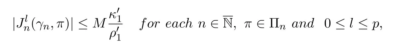
Remark 2.1Under Assumptions 2.1(a)-(c),it follows from Theorem 2.13 in[16]that there exist constantsandfor each 0<τ<2 such that

The expected average criteriafor each givenandare defined as follows:

Definition 2.2(i)For anya policy π ∈Unis called an(constrained)optimal policy of Mnif

(ii)A sequence{φn}withfor eachis said to converge weakly to,if the sequence{φn(·|i)}converges weakly to φ(·|i)in P(A(i))for each i ∈S∞and n ≥n(i).We denote it by φn→φ.

3 Preliminary Results

Assumption 3.1(a)For each i ∈Sn,A(i)is a compact set.

ous in a ∈A(i),for each fixedi,j ∈Snand 1 ≤l ≤p.

(c)There exists a constant M>0,such that|rn(i,a)|≤Mw(i)andMw(i)for all(i,a)∈Knand 1 ≤l ≤p.

Under Assumptions 2.1 and 3.1(c),we can obtain the finiteness of the expected average criteria.

Lemma 3.1[11,16]Suppose that Assumptions 2.1 and 3.1(c)hold.Then

To obtain our main results,we consider the following assumptions:

Assumption 3.2(a)for each i,j ∈S∞,where n ≥max{n(i),n(j)};

Assumption 3.3For eachandthe corresponding Markov process ξtin each model Mnis irreducible.

Remark 3.2(i)Under Assumptions 2.1and 3.3,Theorem 2.5 in[16]yields that for eachand,the Markov chain{ξt}has a unique invariant probability measure,denoted by

(ii)Under Assumptions 2.1,3.1 and 3.3,Theorem 2.11 in[16]implies that the control model(2.1)is uniformly w-exponentially ergodic,that is,there exist constants δn>0 and βn>0 such that

(iii)Under Assumptions 2.1,3.1 and 3.3,for each0 ≤l ≤p and stationary policytheis a constant and does not depend on the initial state i,more precisely,

Assumption 3.4(Slater condition) There exists a policysuch that

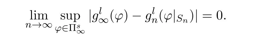
Lemma 3.2Suppose Assumptions 2.1,3.1,3.2(a)-(b)and 3.3 hold.Then,for each 0 ≤l ≤p,

This statement has been established by Theorem 4.21 in[16]for deterministic stationary policies. It is easy to extend the result to the class of randomized stationary policies.

In particular,under Assumptions 2.1,3.1 and 3.3,for eachandNow,we introduce the following sets

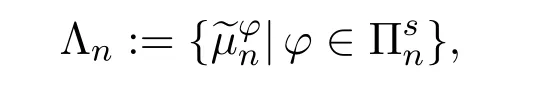
and

Definition 3.1The w-weak topology on Pw(Kn)is the coarsest topology for which all mappings

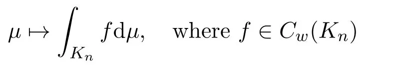
are continuous.

The following lemma characters the w-weak topology;for a proof,see[8,Corollary A.45].

Lemma 3.3A sequenceconverges w-weakly toµif and only iffdµfor every measurable function f which isµ-a.e continuous on Knand for which exists a constant c such that|f|≤c·wµ-almost everywhere.In this case,we write

Lemma 3.4Suppose that Assumptions 2.1,3.1 and 3.3 hold.Then,the set Λnandare convex,compact and closed under the w-weak topology for each

ProofUnder Assumptions 2.1,3.1 and 3.3,it follows from Lemma 8.12 in[16]that Λnis convex and compact. Letwithandby the definition of w-weakly convergence and Assumption 3.1(b),it follows from Lemma 8.11 in[16]that

which implies thatµ∈Λn.Hence,Λnis closed.Furthermore,suppose thatfor each m,then it follows that

for each 1 ≤l ≤p,which implies thatandis closed.Now,suppose thatwe have that

for each 1 ≤l ≤p,which implies the convexity ofThe proof is completed.

Lemma 3.5[10]Suppose that Assumptions 2.1,3.1 and 3.3 hold.Then,for eachthere exists a stationary policysuch thatandfor each 1 ≤l ≤p.

By Assumption 3.4 and Lemma 3.5,there exists a stationary policysuch thatfor each 1 ≤l ≤p. Next,we need to introduce some notations:

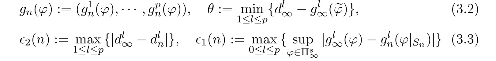
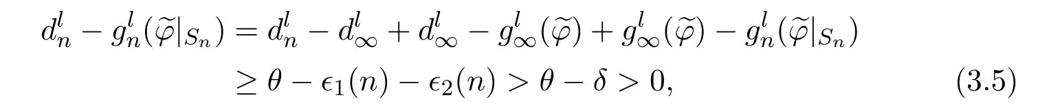
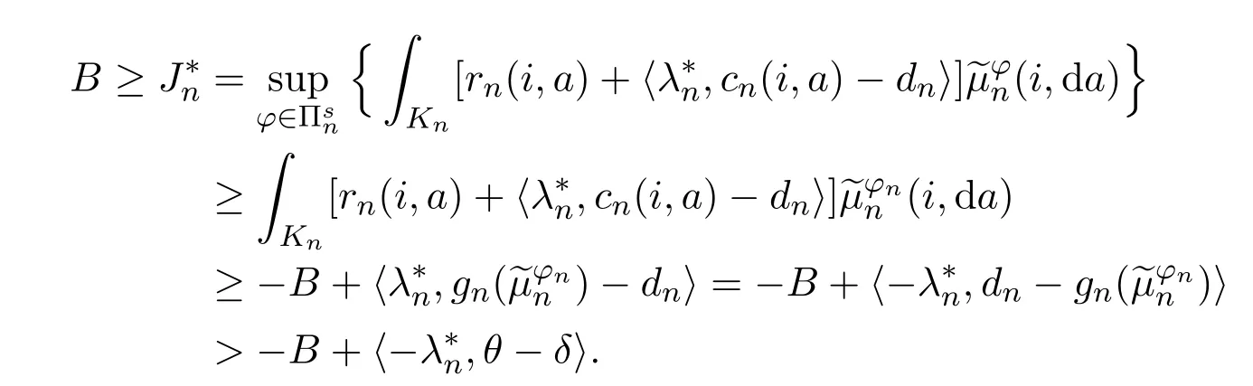
Lemma 3.6Suppose that Assumptions 2.1 and 3.1-3.4 hold,then there exist an integer N∗andfor each n ≥N∗such that

ProofFor each fixed δ<θ,it follows from Lemma 3.2 and Assumption 3.2(c)that there exists an integer N such that for each n≥N,we have ϵ1(n)+ϵ2(n)≤δ and

for each 1 ≤l ≤p.Hence,

The following lemma gives the optimality equation for constrained problem which has been established by Theorem 8.13 in[16]for the case of a single constraint.For completeness,we extend Theorem 8.13 in[16]to any finite numerable of constraints.First,we need to introduce some notations.For each x={x1,···,xp},we defineand say x ≤y if xk≤ykfor each 1 ≤k ≤p.

The proof of the following lemma is similar to that of Theorem 4.10 in[5]for discrete-time MDP,we prove it here only for completeness.

Lemma 3.7Suppose that Assumptions 2.1 and 3.1-3.4 hold. Then,for each

(i)there exist a function hn∈Bw(Sn)and a vectorsuch that

where cn(i,a)−dndenotes the p-dimensional vector whose components arefor each 1 ≤l ≤p;

(ii)there exists a stationary optimal policyof Mn.

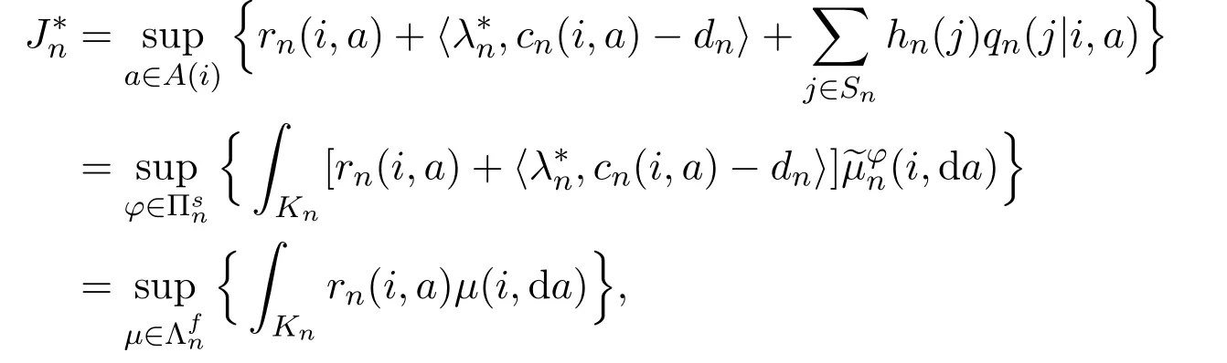
Proof(i)Letbe fixed and

For each z=(z1,z2,···,zp)∈Onwe define

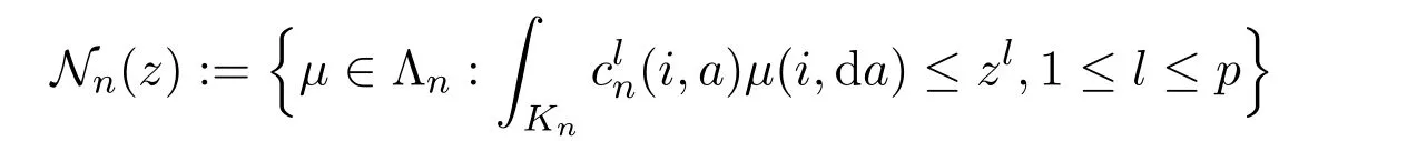
and

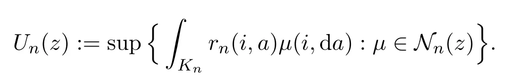
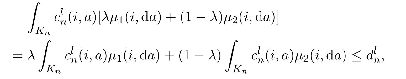
Next,we need to show that Un(z)is concave in z. Let zk∈Onwith zk=for each k=1,2.There existµ1∈Nn(z1)andµ2∈Nn(z2)such thatandLet λ ∈(0,1).We have

and

which implies that λµ1+(1 −λ)µ2∈Nn(λz1+(1 −λ)z2). Thus,it follows that Un(λz1+(1 −λ)z2)≥λUn(z1)+(1 −λ)Un(z2),that is Un(z)is concave on On.

For arbitrary z1,z2∈Onsatisfyingfor each 1 ≤l ≤p,we have Un(z1)≤Un(z2). By Lemma 3.6,dnis the interior of On. Then,it follows from Theorem 7.12 in[1]that there existswithsuch that,for eachTakefor someµ∈Λn.Then,

for eachµ∈Λn.That is,

which implies that

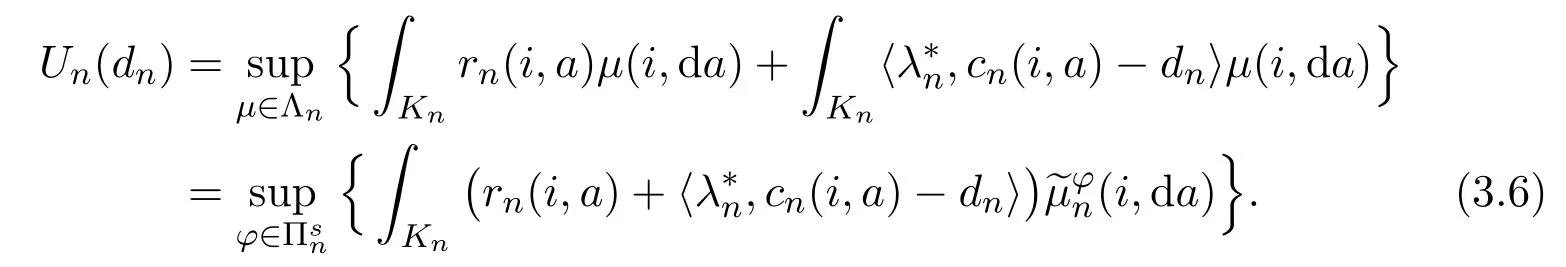
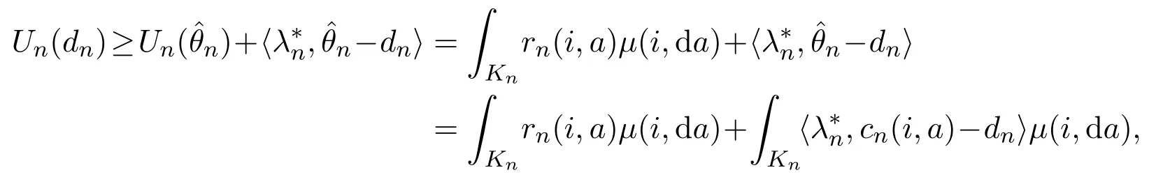
Under Assumptions 2.1,3.1 and 3.3,by(3.6),Theorem 3.20 in[16]and Remark 3.2(ii),there exists hn∈Bw(Sn)such that

for each 1 ≤l ≤p,then we have

On the other hand,by the definition of Un(dn),we haveHence,(ii)LetBy Assumption 3.1(b)and Lemma 3.4,there exist a p.m.and a stationary policysuch that

The proof of the following lemma is similar to that of Theorem 8.14 in[16]with one constraint,we prove it here for the sake of completeness.

Lemma 3.8Suppose that Assumptions 2.1 and 3.1-3.4 hold. Then,for eachthere existandsuch that

ProofLetbe the vector as in Lemma 3.7,we can get the third equality.For each fixedsuppose thatµ∈Λnsuch that the l-th constraints is violated,that isIt follows that

Hence,

which together with Lemma 3.7 implies the first equality.

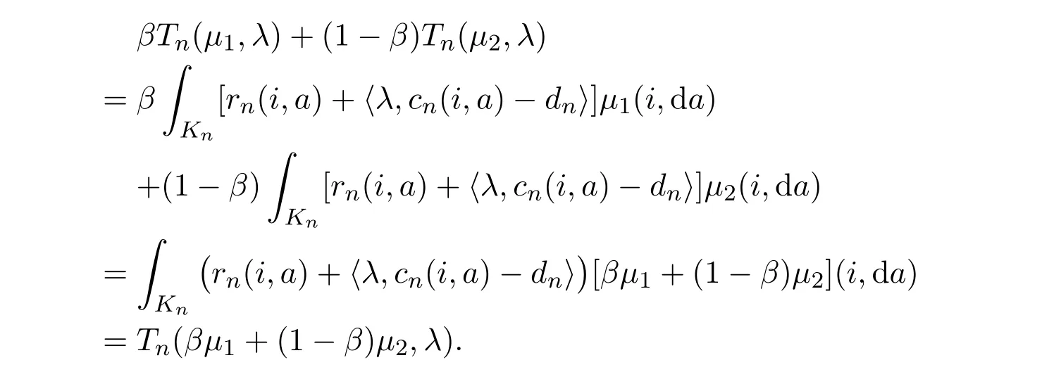
Hence,Tn(µ,λ)is convex inµfor each fixed λ.

which implies that Tn(µ,λ)is upper semi-continuous inµfor each fixed λ.

For each fixedµ∈Λn,let λ1,λ2∈(−∞,0]p.It follows that

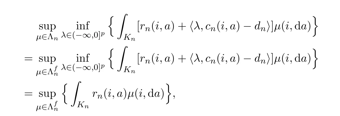
which implies that Tn(µ,λ)is concave in λ for eachµ. By the Minmax Theorem in[2,p.129]or[7,Theorem 2],we have

that is

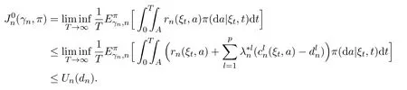
which implies the second equality.By Lemma 3.7,there exists a stationary policysuch thatLet,then

Hence,the last inequality holds.The proof of Lemma 3.8 is finished.

4 The Main Results

Theorem 4.1Suppose that Assumptions 2.1 and 3.1-3.4 hold.Then,

Then,we have

As in Lemma 3.6,there exists a stationary policysuch thatfor each 1 ≤l ≤p.Similarly,we have

which implies that

Under Assumptions 2.1,3.1 and 3.3,by Lemma 3.8,there existssuch that

By(4.1)and(4.3),there existssuch thatLetdenote the restriction of φ in the set Sn,then

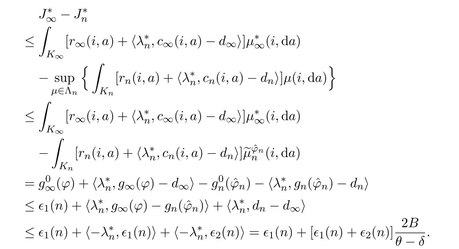
Similarly,by Lemma 3.8,there existssuch that

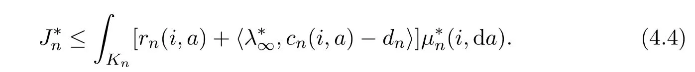
It follows from(4.2)and(4.4)-(4.5)that

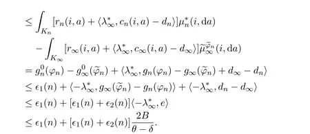
Hence,there exists an integer N such that for eachwhich implies the desired result.The proof is completed.

Lemma 4.1[11]Suppose that Assumptions 2.1,3.1 and 3.3 hold.For any fixedif there existssuch thatthenfor each 0 ≤l ≤p.

Theorem 4.2Suppose that Assumptions 2.1 and 3.1-3.4 hold.Ifis an optimal policy of Mnfor eachand,then φ∞is an optimal policy of M∞.

ProofFirst,we should show that φ∞is a feasible solution of M∞. Letdenote an extension oftoby replacing φnin(4.5)withhere. Under Assumptions 2.1 and 3.1-3.3,by Lemmas 3.2 and 4.1,for each ϵ>0,there exists an integer N such thatandfor each n ≥N and 1 ≤l ≤p.Hence,

which together with Assumption 3.2(c)implies that

for each 1 ≤l ≤p.Hence,φ∞is feasible for M∞.By Lemma 4.1 and Theorem 3.6,we have that

Hence,φ∞is optimal for M∞.The proof is completed.