Clustering in the Wireless Channel with a Power Weighted Statistical Mixture Model in Indoor Scenario

Yupeng Li,Jianhua Zhang＊,Pan Tang,Lei Tian

1 Key Lab of Universal Wireless Communications,Beijing University of Posts and Telecommunications,Beijing 100876,China

2 State Key Lab of Networking and Switching Technology,Beijing University of Posts and Telecommunications,Beijing 100876,China

Abstract: Cluster-based channel model is the main stream of fifth generation mobile communications,thus the accuracy of clustering algorithm is important.Traditional Gaussian mixture model (GMM) does not consider the power information which is important for the channel multipath clustering.In this paper,a normalized power weighted GMM (PGMM) is introduced to model the channel multipath components (MPCs).With MPC power as a weighted factor,the PGMM can fit the MPCs in accordance with the cluster-based channel models.Firstly,expectation maximization (EM) algorithm is employed to optimize the PGMM parameters.Then,to further increase the searching ability of EM and choose the optimal number of components without resort to cross-validation,the variational Bayesian (VB) inference is employed.Finally,28 GHz indoor channel measurement data is used to demonstrate the effectiveness of the PGMM clustering algorithm.

Keywords: channel multipath clustering; mmWave; Gaussian mixture model; expectation maximization; variational Bayesian inference

I.INTRODUCTION

The millimeter-wave (mmWave) spectra is expected to provide unprecedented bandwidth and high-throughput enhancement for the fifth generation (5G) mobile communication systems [1].For deploying the 5G system,one of the key enablers is the realistic channel models.Researchers around the world has contributed to propose feasible channel models for 5G,including the mmWave Evolution for Backhaul and Access model [2] [3],the mobile and wireless communication enablers for the Twenty-twenty Information Society channel model [4],the Third Generation Partnership Project for above 6 GHz channel models [5],and the 5G channel model [6].Being analogous to traditional channel models,these 5G channel models are also cluster-based [7].The clustering of multipath components (MPCs) is of great significance,as it can reduce the modeling complexity and the computational complexity in the technology evaluation.In addition,it has been investigated that channel models,that do not take the cluster into consideration,will overestimate the channel capacity [8].

In the channel field,a cluster indicates a number of MPCs with similar parameters,consisting of the delay (τ),azimuth angle of arrival (AOA),elevation angle of arrival (EOA),azimuth angle of departure (AOD),and elevation angle of departure (EOD) [9] [10] and so on.However,there is no universal definition of MPC cluster,indicating that the clustering results depend largely on how the clusters are identified or modeled.Lots of algorithms have been proposed to implement the clustering,such as.Several algorithms have been proposed to implement the clustering analysis,such as K-means [11],Fuzzyc-means or hierarchical clustering [12],kernel-power-density-based algorithm [13],the novel tracking-based multipath component clustering algorithm [14] and multidimensional power spectra-based algorithm [15] and so on.The Gaussian mixture model (GMM) is employed to fit the MPCs in [10],exhibiting more preferable clustering result compared with traditional clustering algorithms.However,all the above mentioned algorithms do not consider the power information under the statistics framework.In almost all channel model standardizations [16],the MPC power is an important parameter to the channel model.To be specific,in the cluster-based (statistical) channel model,the statistic characteristics of MPC parameters are gotten with MPC power as a weighted factor.A previous algorithm proposed by N.Czink [17] treats MPC power as a weighted factor of a MPC,which accords with the channel model standardizations.In [18] a power weighted GMM is proposed to fit the MPCs.However,the MPC power weighted directly to the Gaussian density function is not reasonable.In addition,ref.[18] must resort to cross-validation methods to determine the optimal number of clusters.

In this paper,we try to use a normalized power weighted GMM (PGMM) to fit the MPCs.As the posterior probabilities of MPCs are mostly less than one,we firstly normalize the inversion of the MPC power.The idea behind the procedure of MPC power is that MPCs with large power will influence the clustering result more than MPCs with small power.Using the PGMM to fit the MPCs accords with the procedure of channel modeling.This is because that,in the statistical channel model,the statistic characteristics of MPC parameters are calculated using MPC power as a weighted factor.Moreover,after proper normalization the power weighted Gaussian distribution can be converted to traditional Gaussian distribution.Then,the PGMM formed by combiningKGaussian distributions can approximate any continuous function very closely,if sufficient Gaussian distributions are used [10] [19].

A powerful method for searching for the maximum log-likelihood estimation of the PGMM parameters is called as the expectation maximization (EM) algorithm [10].By taking the derivation of the log-likelihood function in regard to each parameters,we can get the solving process of the EM-PGMM algorithm.In the expectation step (E-step),we use the parameters to evaluate the posterior probability.In the maximization step (M-step),we use the probability to re-estimate the PGMM parameters.While,EM may fall into local optimization with a high probability.Moreover,EM must resort to cross-validations to determine the optimal number of components.Therefore,variational Bayesian (VB) inference [20] is used to optimize the PGMM parameters.For the VB inference,we can formally find the prior distribution of the PGMM parameters.And then,the variational approximate of the posterior distribution is analytically solved.As sparse prior is added to the mixing coefficients,we can start the mixture model with a large number of components and let competition eliminate the redundant ones.A large number of initial components enables that the VB has a relative strong searching ability.Armed with the VB inference,we can not only avoid overfitting in the procedure of optimization but also determine the optimal number of clusters directly.28 GHz indoor channel measurement data is used to verify the proposed algorithm.

The main contributions of our work are as follows:

1) In order to model the MPCs in accordance with the channel model standardizations,we propose a PGMM.In the PGMM,normalized MPC power are considered as a weighted factor to the Gaussian density function.

2) We use the EM algorithm to search for the maximum log-likelihood estimation of the PGMM.We have derived the EM-PGMM clustering algorithm.

3) Then,the VB inference is employed to further enhance the searching ability of EM and choose the optimal number of components without resort to cross-validation.Besides,with the help of VB inference,the PGMM can effectively avoid overfitting.

This paper is organized as follows.In Section II,the PGMM clustering algorithm is described.In Section III,the EM and VB algorithm are employed to optimize the PGMM parameters,respectively.Indoor channel measurement data at 28 GHz is presented to verify the PGMM clustering algorithm in Section IV.Finally,the paper is concluded in Section V.

Notation:(·)Trepresents the transpose of (·).(·)-1represents the inversion of (·).denotes the Euclidean norm.In this paper,when we usep(·;θ) we deem it as the likelihood function ofθandθrepresents the parameters.In contrary,θrepresents random variables when we userepresents the expectation.

II.THE PGMM CLUSTERING ALGORITHM

2.1 Clustering problem

There are a variety of algorithms to estimate the channel MPC parameters [20].In this paper,we use the space alternating generalized expectation maximization (SAGE) [22] [23] algorithm to estimate the channel MPC parameters,as it can realize the jointly parameter estimation of the channel MPCs.In the channel field,a cluster indicates a group of MPCs with similar parameters [5],including the delay (τ),AOA (φRx),EOA (θRx),AOD (φTx),and EOD (θTx) [10] and so on.Figure 1 illustrates the clustering phenomenon of the MPCs.

In figure 1,the base station (BS) is on the left side,and the mobile station (MS) is on the mobile station.Circles with green dots represent scatters leading to a group of MPCs with similar parameters,called as clusters [10].

In the channel,thenth cluster for the nonline of sight (NLOS) can be modeled as

wherel∈{ 1,2,…L},Lrepresents the number of the clusters,trepresents the time,Mlrepresents the number of MPCs in thelth cluster,Tx and Rx are respectively the transmitting and receiving ends,andare respectively the transmitting and the receiving antenna responses,is the polarization matrix,m= 1,2,… ,Mlis the index of multipath within the cluster,fd,l,mrepresents the Doppler frequency,ntandnrare respectively the transmitting and receiving antenna index,andrepresents the sum of theMlchannel MPCs in thelth cluster.

2.2 The normalized power weighted gaussian mixture model

As is shown in ref.[10],the channel MPCs can be described by a group ofd-dimensional vectorX= {xn;n= 1,2,…,N},wherexn∈Cddenotes the parameters of theith multipath,dis the dimension ofxn,Nis the number of samples.In the GMM,we suppose that eachxnis generated from one of theKGaussian distributions,and the Gaussian distributions model the MPCs as follows

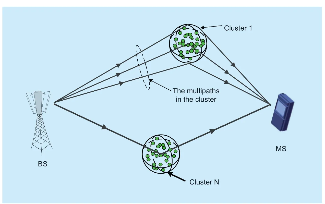
Fig.1.Multipath clustering phenomenon between the BS and MS.

where each component is denoted by the parameters,θk= {µk,Σk;k=1,2,… ,K},µkis the mean,and Σkis the covariance matrix,Kis the number of clusters.In the channel modeling procedure,the MPC power acts as a weighted factor and a MPC with large power will influence the channel modeling more than those with small power.As a fundamental part of statistical channel modeling,a clustering algorithm,in accordance with channel modeling procedure,will benefit the channel model a lot.Thus,we consider MPC power as a weighted factor to the posterior probability of MPC.Then,the posterior probability can be written as

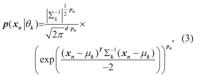
where

wherepn′ isith MPC power.Asin (3) are mostly less than one,a larger MPC power weighted directly to the posterior probability will lead to a smaller value.Therefore,we use (14) to guarantee that a larger MPC power corresponds to a bigger posterior probability.We callpnnormalized power in this paper.

The ML estimation of the PGMM parameters

can be solved by expectation maximization (EM) algorithm.

III.OPTIMIZATION THE PGMM PARAMETERS

3.1 Solving the PGMM parameters with EM algorithm

The EM algorithm,an iterative algorithm,mainly includes two steps.In the E-step,it calculates the posterior probability of the dataset.In the M-step,it re-estimates the parameters that maximizes the PGMM.The relationship of the variables is shown in figure 2,where variables are indicated by circles and parameters are indicated by squares.Node indicated by double circles corresponds to random variables,while nodes indicated by single circle corresponds to hidden random variables.The hidden random variable denotes which component an observed samplexcomes from.The graphic model is shown as below,where the symbolNin the rectangle represents that the variables in it haveNrepetitions.

To search for the PGMM parameters,we get the derivation of (6) in regard to the mean of the PGMM

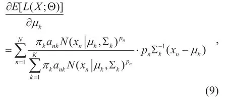
where the Gaussian distribution (3) is used when solving the derivation.We assume

Theznkplays the role of posterior probability.Set (9) to zero,we get

where we defined

whereNkplays the role of effective number of points in clusterk.From the above formula,we can see that the mean of thekth cluster is obtained by a weighted mean of the datapoints in thekth cluster,where the weighted factor of the datapoints are constituted by the power weighted posterior probabilityznk.

Symmetrically,set the derivation of (6) with respect to covariance to zero,and follow a similar reasoning [26],we obtain

where Σkis weighted by the power weighted posterior probabilityznk.

Finally,we maximize (6) with respect to mixing coefficients.Considering the mixing coefficients sum to one and using a Lagrange multiplier,we get

Set the derivation of (14) with respect toπkto zero,we get

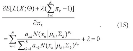
Multiplied withπk,and then summary overk,we get

Substitutingλ=-Ninto (15),we get

In the E-step,we calculateznkwith (10),which calculates the posterior probability.In the M-step,we re-estimate the parameter set of our model with (11),(13) and (17).The signal processing procedure is illustrated in Table I.

3.2 Variational bayesian inference of the PGMM parameters

However,when given a large number of components or the amount of MPCs is small,the EM algorithm could result in overfitting.Besides,to determine the optimal number of components,it must resort to cross-validation [27].

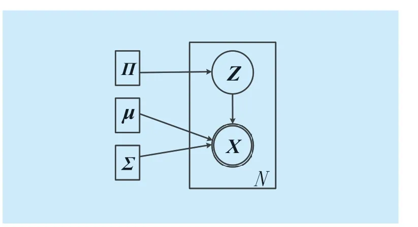
Fig.2.Graphical model for PGMM.

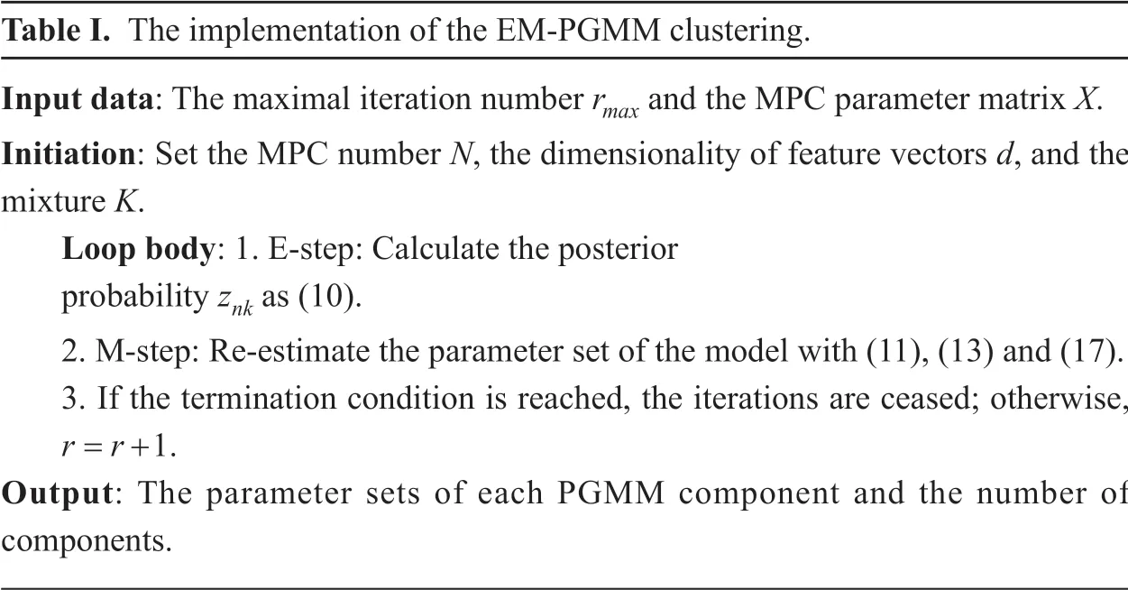
Table I.The implementation of the EM-PGMM clustering.Input data:The maximal iteration number rmax and the MPC parameter matrix X.Initiation:Set the MPC number N,the dimensionality of feature vectors d,and the mixture K.Loop body:1.E-step:Calculate the posterior probability znk as (10).2.M-step:Re-estimate the parameter set of the model with (11),(13) and (17).3.If the termination condition is reached,the iterations are ceased; otherwise,r r= +1.Output:The parameter sets of each PGMM component and the number of components.

To avoid overfitting and determine the optimal number of components,the maximum log-likelihood function is solved by the VB [21].For each observationxn,the corresponding latent variablesznis [z1,… ,zn].Inznone element equals to 1 and the rest equal to 0.Given the mixing coefficientπ,the conditional distribution ofZ[26] can be expressed as follows.

Similarly,knowing the latent variables and the Gaussian parameters,the conditional distribution of the observed data can be expressed as follows

To simplify the expression,we useTkas alternative,whereTkis the precision (inverse covariance) matrix.

For a detailed description of mixing coefficientπ,the Dirichlet prior is used with parametersαk

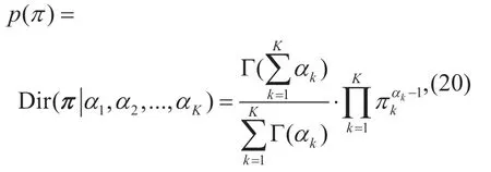
where Γ(·) represents the Gamma function.Serving as parameters of the Gamma function,the same parameterαkis selected for each Gaussian component.The parameterαkcan be interpreted as the prior number of observations associated with each Gaussian component.We setαkto be small values,then the posterior distribution ofπwill be influenced primarily by the observations rather than the prior distribution [26].The Gaussian-Wishart prior is set for (,)µT

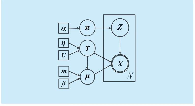
Fig.3.Graphical model for VB-PGMM.

whereUkandηkrepresent the scale matrix and the degrees of freedom,respectively.Serving as multi-dimensional generalization of the Gamma distribution,the Wishart distribution can capture the correlations existing in the MPCs.

The graphical model of VB estimation is illustrated in Fig 3.As Dirichlet prior is added toπand the Gaussian-Wishart prior is added to (µ,T),the seth=(Z,π,µ,T) becomes random variables.α,η,U,mandβserve as parameters that are specified in advance.

Knowing the relationship of the random variables,we can write down the joint distribution,given by

and the logarithm of (23) is

Now we have the latent variablesT,µ,πandZwith the hyperparametersα,ν,V,mandβ.The variational inference scheme can be used to estimate the hyperparameters.We need to calculate the expectation ofL(X,Z,π,µ,T) in (24) with respect to all the other variables apart from the current one.Let us first consider factorZas variables and taking the expectation ofL(X,Z,π,µ,T) with respect toπ,µ,T.The derivation of the update equation is

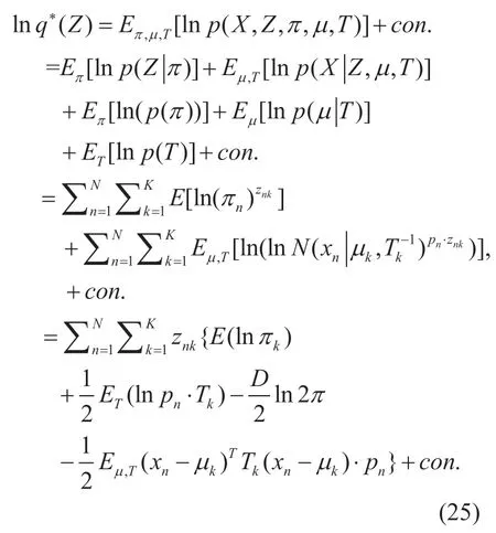
Assuming

we can get

where

Then,consideringπas the variable,the derivation is

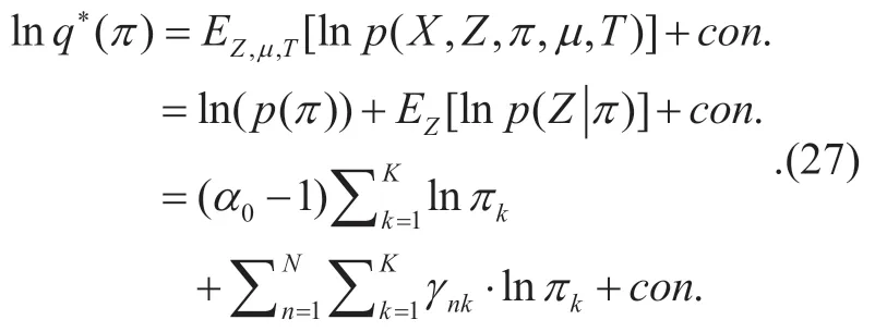
Obviously,(29) has the same shape as the logarithm Dirichlet distribution.Then,q(π) can be expressed as

where

and

Finally,joint distribution ofµandTis

Grouping and reading off terms involvingµkandTk[26],the result is a Gaussian-Wishart distribution shown as

whereνkandVkare parameters of the Wishart distribution representing the degrees of freedom and scale matrix,respectively.Andβk=β0+Nk,where

In the VB inference,the maximum log-likelihood of the PGMM ((28) and (30)) is analogous to the M-step.Calculating the responsibility of the expectation as (26) is referred to as E-step.Then,the solving of the variational posterior distribution involves iterating between two stages similar to the E-step and M-step.The signal processing procedure is shown in Table II.

IV.VALIDATION RESULTS

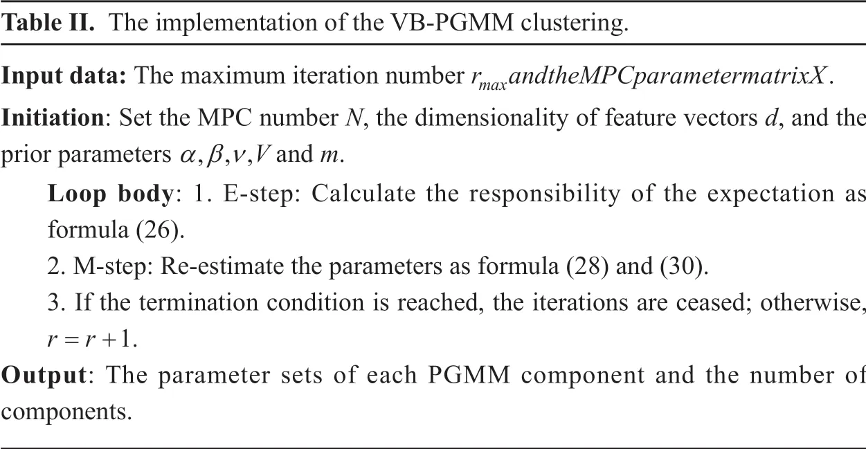
Table II.The implementation of the VB-PGMM clustering.Input data:The maximum iteration number r andtheMPCparametermatrixXmax .Initiation:Set the MPC number N,the dimensionality of feature vectors d,and the prior parameters αβν,,,V and m.Loop body:1.E-step:Calculate the responsibility of the expectation as formula (26).2.M-step:Re-estimate the parameters as formula (28) and (30).3.If the termination condition is reached,the iterations are ceased; otherwise,r r= +1.Output:The parameter sets of each PGMM component and the number of components.

MmWave channel measurement has been carried out all over the world,such as 32 GHz is ourdoor microcellular measurements were conducted in Beijing and so on [28].To compare the performance of PGMM-based clustering and GMM-based clustering,the indoor channel measurement data at 28 GHz is used.To search for the optimal parameters of traditional GMM,the EM algorithm and VB algorithm are respectively used to derive the EMGMM clustering algorithm and the VB-GMM clustering algorithm.Parallel,the EM and VB algorithm are respectively used to search for the PGMM parameters deriving the EM-PGMM and VB-PGMM clustering algorithm.

Table III.28 GHz measurement configurations.

Fig.4.The panorama of the indoor measurement environment.

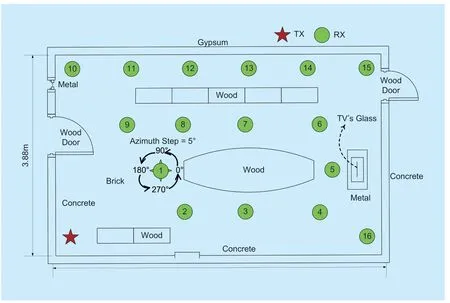
Fig.5.Detailed exhibition of measurement environment.

4.1 Measurement scenario

In the measurement,the correlator channel sounder is used with 600 MHz bandwidth at 28 GHz.Transmitter and receiver are synchronized by the same reference clock source.To achieve well dynamic range in the link budget,the low noise amplifier (LNA) and power amplifier are respectively used at transmitter (Tx) side and receiver (Rx) side [1].

The measurement campaign is conducted in the Beijing University of Posts and Telecommunications (BUPT),the overall perspective is presented in figure 4.It is a typical indoor conference scenario with the geometric size of 10.97 ×6.62 ×2.40m3.figure 5 shows that Tx is fixed at the corner of the room and Rx side is located at various locations in the room.The antenna is about 1.55 m height for both Rx and Tx.

The detailed setup of the measurement is as follows:Rotating the horn antenna (25 dBi,10°(horizon power bandwidth) HPBW,11°(elevation power bandwidth) EPBW) at Rx over azimuth-elevation pairs successively,and an omni-directional antenna (2.93 dBi) is used at Tx.In the elevation angle of respectively 10°,0°and -10°,the Rx collects 72 samples in the azimuth angle with the step of 5°.In this way,MPCs from different directions could be recorded independently and the parameters in the spatial domain can be analyzed.The key configurations are listed in Table III as a summary.

Then,the virtual circular array receiver by rotating the horn antenna are obtained.The virtual circular array receiver is similar to the real circular array receiver in the theoretically [1].Figure 6 illustrates the layout of the virtual array measurement scenario.

4.2 Parameter settings

After channel parameter estimation using the SAGE,we get 100 multipaths and their corresponding parameters.As the omnidirectional antenna is selected at the Tx,there is notφTxorθTx.The input data dimensiondis 4,that is [τ,φTx,θTx,power].The dataset is arranged in column asX= (x1,x2,… ,xN),wherexj= (xj,1,xj,2,…,xj,d) represents thejth (j=1,2,… ,N) multipath vector.The diagonal covariance matrix is chosen for the Gaussian distribution.

4.3 Choosing the optimal number of components

With the increase of cluster number,the model will fit the dataset more precisely.Then,the log-likelihood increases monotonically with the increase of components.While,too many components will lead to a high model complexity.Besides,choosing too many components will lead to an overfit of the data [29].So we need to make a trade off between the model complexity and the fit degree of the dataset.In the VB inference,an approach to choosing the optimal number of components is to treat the mixing coefficients as parameters.Then,we can make a point estimation of the mixing coefficients.The detailed description of the estimation is

The update of the mixing coefficients is interleaved in the variational update of the other parameters.As sparse prior is added to the mixing coefficients,the mixing coefficient will tend to zero during the iteration if the corresponding component provides little contribution to fitting the dataset.Besides,is several components fall into the same area in the space,the model tends to eliminate the redundant ones.Therefore,we usually initialize a model with a relative large value ofKand let the redundant components be pruned out automatically.This mechanism enables that VB-PGMM possesses relative strong searching ability.

4.4 Clustering comparison between GMM and PGMM

4.4.1 Clustering comparison under the validity index:

There are a variety of cluster validity indices,i.e.,the Davies Bouldin (DB) index,the Beni index,SV index,and Pakhira Bandyopadhyay Maulik index,to evaluate the reasonability of the clustering result [27].Generally,these validity indices reach a uniform conclusion.Here,we use the DB index [29] as an example.We simulate 100 channel sampling snapshots.The results are shown in figure 7.

In the channel MPC clustering,a low DB value is preferable,which corresponds to an intra-compact and inter-separate clustering result.From figure 7,we can see that the DB values of the VB-PGMM clustering algorithm are the lowest among the four clustering algorithms.And EM-PGMM also gets a better performance than the EM-GMM and VB-GMM clustering.This attributes to the superiority of PGMM which provides reasonable explanation for the MPC power.As VB inference initializes with a relative largeKvalue and eliminate the redundant ones during the iteration,VB-PGMM clustering possesses a relative strong global searching ability.So VB-PGMM gets a relative stable DB values compared with EM-PGMM.Compared with the above two clustering algorithms,VB-GMM and EMGMM get relative poor performances.Considering both mean and variance information of the dataset,GMM-based clustering framework can get more preferable clustering result than Kmeas (KPowerMeans)-based framework,which has made detailed analysis in ref.[9]-[10].

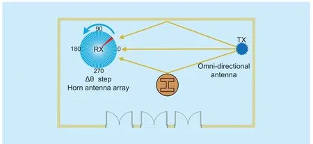
Fig.6.Layout of the virtual circular array measurement.

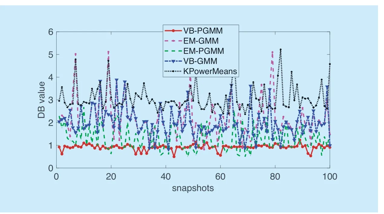
Fig.7.The DB values of different algorithms in different snapshots.

4.4.2 Clustering comparison in the visual aspect:

To enlighten the influence of MPC power on clustering,we choose MPC power as a factor for the visualization.Therefore,the 3 parameters we choose for the visualization is the delay,power,and EOA.Figure 8 and figure 9 illustrate the visualization comparison in 5 clusters,where the same cluster is colored the same.

In the visualization,different clusters have clear boundary with each other is preferable,as intra-compact and inter-separate clustering result is expected.A clustering result with clear boundary represents that the corresponding clustering algorithm has strong resolution ratio in these dimensions.As can be seen from figure 8 (a) and figure 9 (a),EM-GMM and VB-GMM clustering algorithm get chaotic clustering result,especially among [100,300] in the delay dimension.Conversely,in figure 8 (b) and figure 9 (b),the PGMM-based clustering algorithm gets relative clearly clusters.Especially,in the VB-PGMM clustering algorithm the result has clear boundary.This demonstrates that,with the help of power,the PGMM can reveal the inner structure characteristics of MPCs successfully.MPC power is an important factor in the channel modeling.The PGMM-based clustering technique conforms closely to the cluster-based channel model,which will contribute to the improvement of channel modeling precision.

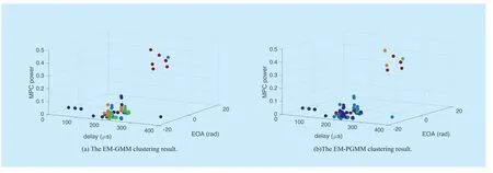
Fig.8.The comparison of EM based GMM and PGMM in the visual aspect.

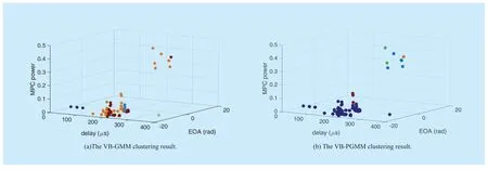
Fig.9.The comparison of VB based GMM and PGMM in the visual aspect.

V.CONCLUSION

In this paper,we demonstrated that GMM can not correspond with the procedure of channel modeling reasonably.To overcome the problem,a PGMM clustering framework is proposed to model the channel multipaths.In the PGMM,MPC power is considered as a weighted factor to the posterior probability,enabling that the PGMM fits the MPCs in accordance with the statistical channel models.To search for the PGMM parameters,the EM algorithm is used.Then,to enhance the searching ability of EM,the VB inference is employed.In accordance with the channel propagation characteristics,the PGMM clustering algorithm is expected to obtain favorable clustering result.In the simulation,28 GHz indoor channel measurement data is used to demonstrate the effectiveness of the PGMM clustering algorithm.The validation results illustrate that VB-PGMM clustering algorithm can obtain the favorable performance from quantitative aspect.In the visualization aspects,the VB-PGMM clustering can get clusters with clearly boundary.As VB-PGMM technique conforms closely to the statistical channel model standardization,we have sufficient confidence to obtain a channel model with improved precision.

ACKNOWLEDGEMENTS

This research is supported by National Science and Technology Major Program of the Ministry of Science and Technology (No.2018ZX03001031),Key program of Beijing Municipal Natural Science Foundation (No.L172030),Beijing Municipal Science ＆ Technology Commission Project (No.Z171100005217001),Key Project of State Key Lab of Networking and Switching Technology (NST20170205),and National Key Technology Research and Development Program of the Ministry of Science and Technology of China (NO.2012BAF14B01).