EEG Source Localization Using Spatio-Temporal Neural Network

Song Cui,Lijuan Duan,2,Bei Gong,＊,Yuanhua Qiao,Fan Xu,Juncheng Chen,Changming Wang

1 Faculty of Information Technology,Beijing University of Technology,Beijing 100124,China

2 Beijing Key Laboratory of Trusted Computing,National Engineering Laboratory for Critical Technologies of Information Security Classified Protection,Beijing 100124,China

3 College of Applied Sciences,Beijing University of Technology,Beijing 100124,China

4 The National Clinical Research Center for Mental Disorders ＆ Beijing Key Laboratory of Mental Disorders,Beijing Anding Hospital,Capital Medical University,Beijing 100088,China

5 Advanced Innovation Center for Human Brain Protection,Capital Medical University,Beijing 100069,China

Abstract: Source localization of focal electrical activity from scalp electroencephalogram (sEEG) signal is generally modeled as an inverse problem that is highly ill-posed.In this paper,a novel source localization method is proposed to model the EEG inverse problem using spatio-temporal long-short term memory recurrent neural networks (LSTM).The network model consists of two parts,sEEG encoding and source decoding,to model the sEEG signal and receive the regression of source location.As there does not exist enough annotated sEEG signals correspond to specific source locations,simulated data is generated with forward model using finite element method (FEM) to act as a part of training signals.A framework for source localization is proposed to estimate the source position based on simulated training data.Experiments are done on simulated testing data.The results on simulated data exhibit good robustness on noise signal,and the proposed network solves the EEG inverse problem with spatio-temporal deep network.The result show that the proposed method overcomes the highly ill-posed linear inverse problem with data driven learning.

Keywords: electroencephalogram; LSTM; source localization; spatio-temporal modeling

I.INTRODUCTION

ELECTROENCEPHALOGRAPHY (EEG) is a popular technology that records the dynamics of the neural activity,which is widely used in both clinical research and treatment.Among all EEG collections,scalp EEG (sEEG) is more common in diagnosis,because of its non-invasive,safety,convenience and low price.Moreover,in studies like brain-computer interfaces (BCI),brain state in cognition process and diagnosis of neurological diseases,sEEG signal has an advantage of high temporal resolution.However,the spatial information in sEEG have not been fully developed.Exploring EEG source localization continues to be a meaningful topic in EEG research [1].

According to the assumption of dipole sources,two categories of methods for localization are proposed.When dipole number is given,a direct method for localization is to simulate the signal conduction and find the group of sources that could generate the most like signal with real sEEG.Dipole fitting methods [2,3] are the most common approaches for source localization modeling the source with a few equivalent current dipoles (ECDs).The method is feasible for focal source localization in clinical treatment,especially the localization of magnetoencephalogram (MEG) sources.When the number of EEG sources is unknown,a series of methods for EEG source imaging (ESI) are proposed to estimate the distribution of source dipoles.The source localization problem is described as linear inverse problem.To explore the unique solution of the inverse problem,constraints are given based on the characteristics of actual source distribution.One of the classic method to describe the unique solution of the inverse problem is minimum norm estimate (MNE) [4],which minimizing the energy of source activity withL2-norm.Weighted MNE (wMNE) [5] and low-resolution electromagnetic tomography (LORETA) [6-8] are also proposed based onL2-norm of the source that incorporate some spatial information.Generally,methods based onL2-norm perform better on extended sources imaging.To improve the performance on focal sources,sparsity constraints are introduced in EEG inverse problem [9-11].It is found that estimations could concentrate on more focal sources withL1-norm sparse regularization.Although these estimations reduce the searching space using constraints,the inverse problem is still illposed.Besides,these approaches are nonsmooth and noise sensitive since it locates the source activity with instant sEEG.

In fact,temporal information is crucial for source activity reconstruction.Firstly,adjacent time signal provides more measurements to the ill-posed linear problem.These measurements make the inverse problem easier to solve by compressing the solution space.Secondly,there are some sequential patterns in EEG signals that describing the source activity and helping the reconstruction.For example,oscillation of sEEG signal is related to the location of sources,and the amplitude of the source signal is decayed with the depth of sources.Moreover,temporal dynamics modeling of sEEG signal decreases the noise influence and makes the estimations of source smoother in time.To introduce temporal information,first and second-order derivatives with time are incorporated to the optimization [12,13].However,the constraints of temporal information still need to be reinforced,and statespace models like multivariate autoregressive (MAR) are also introduced [14,15].Although,the ability for representing EEG from time perspective is improved,MAR shows less capacity for representing some waveforms,such as event related potentials (ERPs).Several other recent approaches [16-20] models the temporal information with predefined or data-driven temporal basis functions (TBFs) in M/EEG source reconstruction.Then,the source activity is solved by an alternative process between TBFs and spatial basis.In general,temporal information is helpful in confining the solution space of inverse problem,and the model that is closer to realities provides solution that is more accurate.

For both spatial and temporal modeling,the accuracy of these methods are decided by the exactness of model assumptions.However,human brain is a delicate and complicated “machine”.The existing method still needs to be improved to model the neural connection and signal processing completely.Moreover,most of the present approaches are based on simplified neural activity simulating mathematical model making the localization based on dipole modeling less performable in some aspects.Indeed,representing the brain activity with simple model is less effective than fitting the relationship between sEEG and source activity with a complex optimization.In some early researches [21-24],artificial neural network (ANN) is used to reconstruct the source localization in MEG and sEEG.The network model used in these approaches are basic ANN neglecting the temporal information in source localization.Many researches show that deep learning methods are also helpful in dealing with ill-posed inverse problem [25-28].However,solving the EEG inverse problem with deep learning methods is still a very promising field.

With the improvement of better optimization methods,hardware devices and learning strategies,learning a complicated model with numerous parameters becomes possible.In recent research [29],convolutional neural networks (CNNs) is used to localize source for premature ventricular contraction from 12-lead electrocardiogram (ECG) which confront similar ill-posed inverse problem.In fact,different network structures can learn different information in signal.For example,recurrent neural network (RNN) [30,31] is effective in learning sequential signal.Longshort term memory recurrent neural networks (LSTM) [32-34] is one of the improvement for RNN.By introducing several gate operations,the network can learn when to forget the past states and when to update current states considering the current inputs.These improvements make LSTM networks not affected by error vanish,and possible to learn long-term dynamics.Meanwhile,EEG signal usually containing a long-term dynamic.The characteristic of EEG fit in with the advantage of LSTM network.Therefore,in the proposed approach,LSTM networks is chosen to learn spatial-temporal information in EEG signal for its proven effectivity in learning long-term dynamics.

Nowadays,with more abundant data and more powerful machine learning methods,spatio-temporal information can be learned effectively from generous sEEG signal as the relation between sEEG and source activity is a complicated mapping function.Data driven learning is promising to solve the inverse problem not confined by linear model and constraints.

In the proposed model,we build the function between sEEG signal and the parameters of source location by spatio-temporal neural network.The contribution of this paper includes:

1) A new idea in solving spatio-temporal EEG inverse problem is provided in the proposed approach.Rather than mathematic modeling with strong priori hypotheses,the inverse problem is modeled with data-driven spatio-temporal neural networks.Therefore,a framework for source localization is proposed to estimate the source position.

2) According to the requirements for modeling EEG inverse problem,the sequence to sequence LSTM network is used as the spatio-temporal neural networks.Moreover,the problem is well resolved by encoding the spatio-temporal information and decoding the source location with the sequence to sequence LSTM network.

3) Experiments on simulated data show the effectiveness of the proposed method.The proposed method shows its advantage on robustness of noise.

The rest of this paper is organized as follows.In Section II,the background of spatio-temporal EEG forward problem is described in details.In Section III,we proposed a spatio-temporal neural network to model the inverse problem.In Section IV,experiments and results on simulated data are provided.In the end,some conclusions are given in Section V.

II.BACKGROUND

2.1 EEG forward problem

The EEG forward problem is to estimate scalp EEG signal with known source activity.The basic forward problem is modeled without temporal information in EEG signal.In mathematical formulation,the relationship between source neural activity and the measured scalp EEG is usually considered as a linear model:

wheretis the time,lt∈Rd×1is the recorded EEG measurements fromdelectrodes on scalp;H∈Rdn×is the conduction matrix that reflect the correlation between n distributed sources and sensor EEG activity;st∈Rn×1is the signal from sources,and ∈t∈Rd×1is the noise from observation.

If the source activity is obtained,the acquisition ofHis critical for the forward problem,andHis obtained by modeling magnetic resonance imaging (MRI) using finite element method (FEM) or boundary element method (BEM).In this model,the spatial structure is efficiently considered.However,the impact of the timetis neglected,and the conduction from sources to sensors on scalp is linear with fixed time.

Recently,time influence is considered [17],and sources activity is represented using spatial basis and temporal dynamics.It is given as follows:

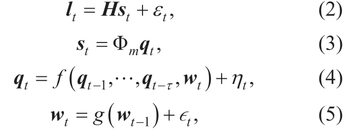
where Φm∈Rn×cdenotes a set of spatial basis andqt∈Rc×1denotes coefficients on each spatial basis to represent source activityst.As the spatial basis has been factored out,neural activityqtis described byf(⋅) to simulate the temporal influence of neighbor state evolution over time periodτ.wtdenote parameters of functionfwhich is modeled as random walk processg(⋅).

In this model,the precision of conduction matrixHis affected by segmentation of MRI and head model construction method.It brought a high computation complexity to get an accurate conduction matrix.It is also assumed that the influence of head model on source signal is linear.However,the neuron connection and many other principles of the brain are still uncovered.

III.METHOD

3.1 Forward problem for neural network modeling

The mathematic modeling needs some assumptions to simplify the model for calculation.However,for neural network modeling,the only assumption is that there is a function between source signal and measured EEG signal.

Therefore,we use functionhto represent the conduction process and scalp signal generated by functionhact on source activity,and it is given as:

The functionh(⋅) may be non-linear and contains spatial and temporal information from source signalst-τ,… ,st-1.

3.2 Modeling inverse problem with spatio-temporal networks

1) From Bayesian modeling to networks modeling inverse problem

For EEG inverse problem,following Bayesian framework [10],the reconstruction of neural activity can be represented as the calculation of the condition distributionP(st|lt-m,lt-m+1,… ,lt).According to the posterior probability formula,the distribution of sourcestunder observationlt-m,lt-m+1,… ,ltis represent as follows.

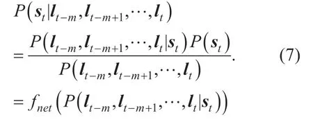
P(lt-m,lt-m+1,… ,lt|st) is the measured signal under sourcestwhich is the observation on scalp.P(st) andP(lt-m,lt-m+1,… ,lt) represent the priori distribution in spatial and temporal respectively.In traditional method,P(st) is modeled with assumption of head model andP(lt-m,lt-m+1,… ,lt) is modeled with MAR or TBFs.Thus,in this approach,assuming that these priori knowledge can be represent using functionfnet()⋅.Following the idea of learning methods,when the amount of source activity and scalp EEG is huge enough,the functionfnetbetween source activity and measured signal can be learned.We approximate the functionfnet()⋅ using neural networks.In this way,the priori knowledge need not to be given empirically.It is learned from training samples and implicated in the neural networks.Moreover,the network should have the capacity for learning both spatial and temporal information from EEG signal.

2) The framework for modeling inverse problem with spatio-temporal networks

Although the sEEG collection is common in clinical research,the sEEG with label indicating the source is still difficult to obtain.Therefore,a framework is proposed to estimate the source position based on simulated training data.The flowchart is given in figure 1.The process contains two phase,training and testing phase.In training phase,traditional forward model is used for the generation of simulated signal and the head model is obtained from the segmentation of MRI data.The electrodes position is aligned and matched in the head model.Moreover,the source activities including position,dipole moment and source signal are settled based on source estimation.For source position,the source is among the position of white and gray matters.To make the network more robust,noise is added to the generated signal.The network can learn how to deal with noise from the abundant mixed training signals.With simulated sEEG signal and source position,the networks are trained to locate the source position.To test the trained neural networks,the testing sEEG signal is input into the networks to estimate the source location.

3) Representing spatial and temporal information with LSTM

To model the relation between sEEG and source signal,sequence to sequence network in [33] is used.Sequence to sequence LSTM network is a type of deep artificial neural networks that learns information from input sequence and decode the learned information with the structure of outputs.It is selected because the encoder network can model the spatio-temporal information from EEG signal and the decoder network can decode the source location.Similar with other supervised learning algorithms,original signal and expected label for training samples are fed into the network.The weight in the network are trained to solve the inverse localization problem.

The network contains two pathways to model combination of information from sEEG and source signal.For sEEG encoding,an LSTM is used to learn the spatial and temporal information from sEEG signal.For source decoding,the source location is decoded from implicit location in hidden layers of LSTM.

The network structure is given in figure 2.

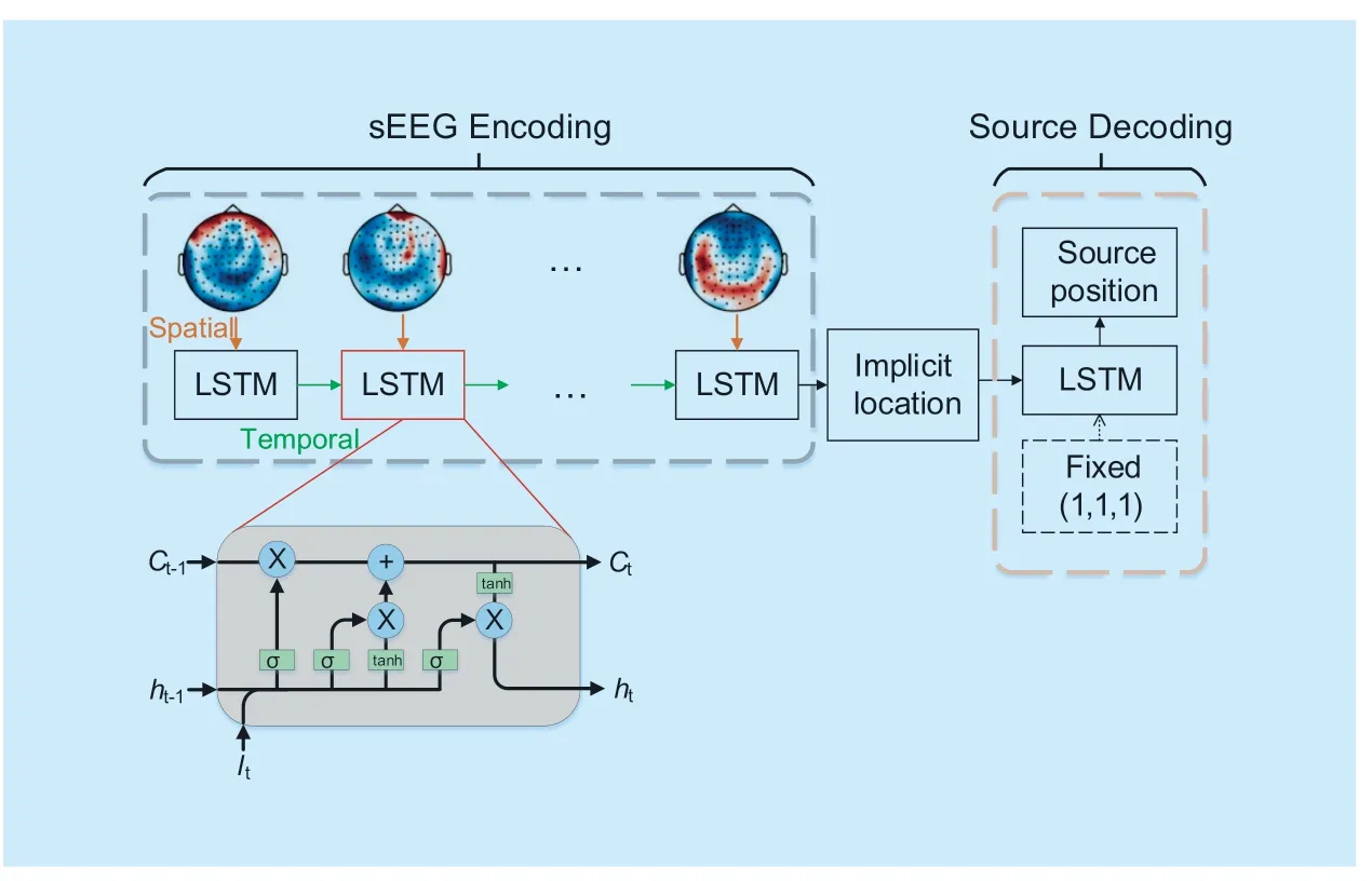
Fig.2.Network architecture for EEG inverse localization problem.

First,the input of the network is a sequence of sEEG signallt,1,,tT=… ,where eachlt∈Rd×1contains the voltage fromdelectrodes.Second,the LSTM extract the latent representation of sEEG sequence into a hidden layer.In each time step,hidden nodes are connected with both input nodes and itself in last time step.Following the LSTM unit in [34],for inputltat timet,the hidden statehtrepresent the current state with following steps:

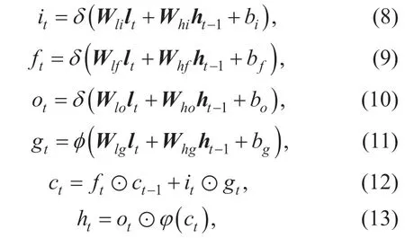
whereδ()⋅ andφ()⋅ are non-linear sigmoid and hyperbolic tangent function,respectively;Wrepresent the weight matrices between subscript layers and gates;brepresent the biases of subscript gates; ⊙ is the element-wise product for gate value.In addition,itindicates the input gate,ftis the forget gate,otindicates the output gate,gtis the input modulation gate,ctis the memory cell andhtis the hidden unit.With the weights onit,ftandot,LSTM learns how much input and memory cell should be preserved and how much memory cell to be transferred.These gates make LSTM flexible to learn signal that is extremely complicated and the long-term dynamics.ltdenote signal collected in every channels.As shown in figure 2,the input layerltand hidden layerhare fully connected; the weight matricesWexpress the relation between electrode and sources.For given sEEG signal at stept,LSTM extract the spatial and temporal information in hidden layerht.In Eq.8-11,the spatial information is learned and remembered in the weightsWl*between input and hidden layer.By connecting the previous hidden layer,the temporal information is hidden in the weightsWh*.The network uses a LSTM with 784 hidden nodes.

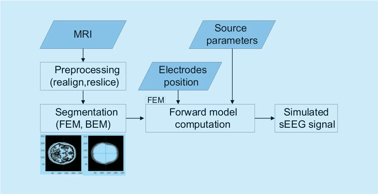
Fig.3.The flowchart of simulated sEEG signal generation.

In source decoding stage,the network is an LSTM with single time step.The decoding network uses implicit state from encoding LSTM as initial state of hidden layer.The hidden layer is then fully connected with output nodes,which is the location parameters of the source.Moreover,a fixed location (1,1,1) is used as the input of source decoding.The proposed approach tries to find the parameters with regression of source coordinates.Therefore,mean square error (MSE) is used as the loss function of the networks.

wherexi=(lt-m,lt-m+1,… ,lt) denotes theith series of sEEG input,yidenote the source position ofith input,andNdenotes the sample number.

IV.EXPERIMENTS

For the neural network,source information is acquired from the generated data.Therefore,the generated data should be close to real situations and the networks should be able to approximate the solution of inverse problem.In this section,experiments are done to verify the performance.

4.1 Generating signal using forward model

For the modeling of forward problem,the generation of simulating signal is obtained using Fieldtrip toolbox [35].This sEEG signal generating process requires three main parts,the head model,the electrodes position and the source signal parameters.First,for the construction of head model,FEM is selected to make the generated signal more similar with real EEG signal as it provides more accurate head model than BEM approach.By segmenting the MRI of a standard brain,the head is segmented into scalp,skull,cerebrospinal fluid,gray matter and white matter,and the conductivity are 0.43,0.0024,1.79,0.14,0.33,respectively.The conductivity of different tissues is set following the studies on cortex stimulation [36,37].Second,to make the electrodes position for generated signal the same with testing EEG signal,standard BIOSEMI-128 EEG system is used for signal generation.Third,as three parameters,source position,source dipoles orientation and source activity are related to source signal properties.In each generated signal,the parameters are set varied to make the network more generalized and robust for different situations of source.Therefore,the source position is randomly selected from the position of gray/white matters containing neurons.The dipole orientation is also set stochastically for different generated signals.For the source activity,the generated source is added with white noise.The flowchart of the simulated sEEG signal generation is shown in figure 3.

4.2 Experiment on stationary simulated data

The stationary simulated signal is first used for the experiment to show the performance of the proposed approach.We have generated 15000 and 1000 simulated single source signals with different positions for training and testing,respectively.Each signal is a one-second segment with 250 Hz sampling rate and 128 channels located by the standard BIOSEMI-128 EEG system.In the training set,for every source location,three simulated signals with different source dipole orientation are generated.For testing set,source parameters are different from each other.In our experiment,stationary brain activity generation is based on the model in [17],shown as follows:

wherexkis the source signal value in timek,and the parameter values areτ=20,a1=1.0628,a2=-0.42857,a3=0.008,a4=0.000143,a5=-0.000286 and≤0.05.As the firstτtime steps for source signalxkare random,the generated stationary signals are different from each other.

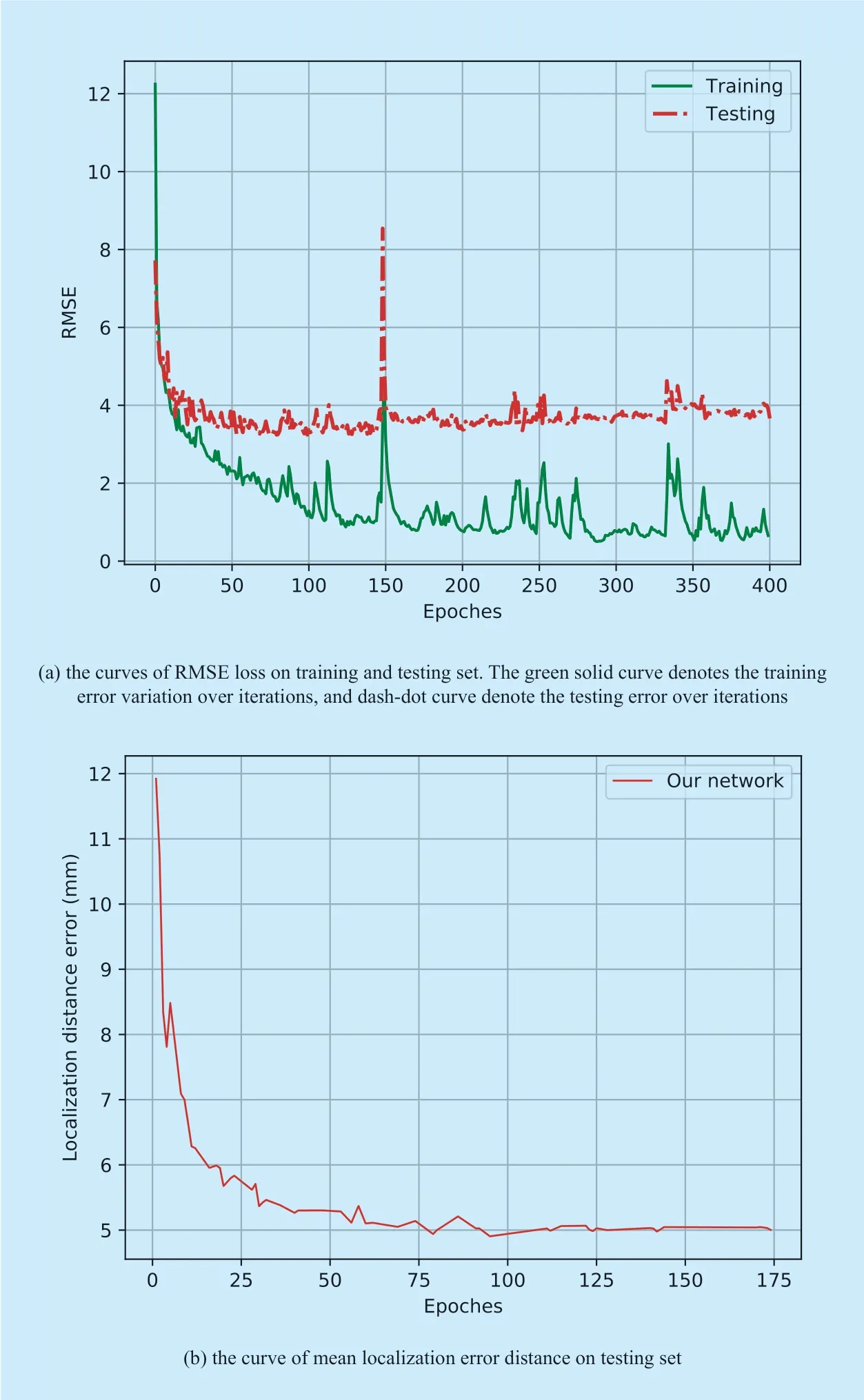
Fig.4.Performance of proposed network.

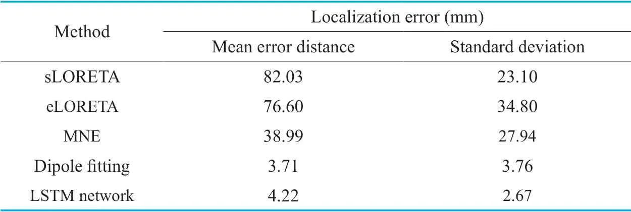
Table I.Localization result compare with different methods.

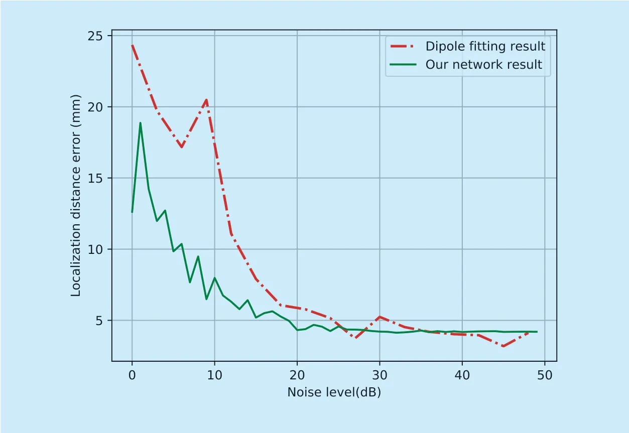
Fig.5.Noise influence of the proposed approach and dipole fitting.

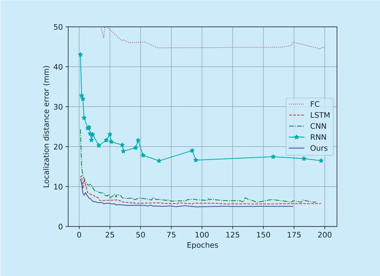
Fig.6.Localization error distance with different networks.The magenta dot line is the result of FC network (44.31mm); the red dash line is the result of a single layer LSTM network (5.57mm); the green dash-dot line is the result of a CNN network (6.06mm); the cyan dash-star line is the result of a single layer RNN network (16.43mm); the blue solid line is the result of the proposed network (4.90mm).

The proposed approach estimates the source location with coordinate regression.Therefore,the performance is evaluated using distance between estimated position and ground-truth position on the simulated data.The position of dipole is given by CTF coordinate system.The network is trained on training set with 400 epochs.In figure 4,the performance of the proposed network over the iterations are plotted.As shown in figure 4(a),after several iterations,the training and testing error curves converge to a low level.Meanwhile,the network shows good generalization on testing set.The mean localization error distance of optimal model on testing set is 4.90±3.55 mm.

The result is compared with some other traditional methods for source imaging and dipole fitting.As the time consumption of traditional methods is huge,twenty testing samples are selected stochastically to evaluate the performance of different methods.For source imaging methods including sLORETA,eLORETA and MNE,the position with maximum mapping value is used as the predicted source location.The result is shown in Table I.From the results,it is observed that the localization error distance of sLORETA,eLORETA,MNE are both greater than 30 mm.Dipole fitting,and the proposed networks localize the dipole with distance less than 5 mm.As source imaging approaches give an approximate area of the source,it predicts the focal source in lower precision by estimating dipoles all over the brain.The experiment also shows that the LSTM network do solve the EEG inverse problem.

1) Influence of noise

In this section,different degrees of noise are added to the simulated signals to evaluate the robustness of the proposed approach.White noise is added into every channels of the simulated sEEG signal,and the signal-tonoise ratio(SNR) of signal is set to be 0-48 dB.The lower SNR means the power of noise is stronger.For the proposed approach,the noisy sEEG signal is directly tested with the optimal model that trained by clean simulated signal.The result of the proposed approach and dipole fitting on noise signal is shown in figure 5.It can be observed that the proposed approach maintained lower localization error distance than dipole fitting when the noise is strong.As the real EEG signal usually contains strong noise,the performance in lower SNR is more important.Therefore,the proposed approach shows greater robustness than dipole fitting.The biggest gap between the proposed approach and dipole fitting is about 15 mm.And when the SNR is higher than 25 dB,the localization error distance of these two approaches keep in the same level.

2) Performance on different networks

According to previous research [21,22] on solving EEG inverse problem with neural networks,fully connected network can also solve the problem.Moreover,CNN structure can solve ECG localization problem as in reference [29].Therefore,a VGG-like network [38] is also used as a comparison with the proposed method.In this section,the results of fully connected network (FC),single layer LSTM network (LSTM),single layer RNN network (RNN),VGG-like convolutional neural network (CNN) and sequence to sequence LSTM network (Ours) are compared.The tested fully connected network is a two-layer network with 784 hidden nodes for each hidden layer.It contains 26.29 million trainable parameters in total.The single layer LSTM network contains a hidden layer with 1024 hidden nodes with 4.73 million trainable parameters.As for the single layer RNN network,the number of hidden nodes is 2048.Thus,4.46 million trainable parameters are settled.The CNN network contains seven convolution layers with 3×3 receptive fields,three max-pooling layers and two fully connected layers.MSE between the prediction and the ground-truth source location is used as the loss function.There are 9.81 million trainable parameters in the network.The proposed network contains two hidden layers with 784 hidden nodes,one is for the sEEG signal encoding and the other is for the source decoding.The trainable parameter number for the proposed network is 5.30 million.The result is given in figure 6.The optimal results for fully connected network,single layer LSTM,CNN,single layer RNN and sequence to sequence LSTM network are 44.31,5.57,6.06,16.43 and 4.90 millimeter,respectively.Fully connected network have the largest trainable parameters,the localization error distance is significant larger than all the other networks.With similar trainable parameters,the result of LSTM based network is significant better than RNN.It indicates that when facing the long-term EEG dynamics,the LSTM network present better performance than RNN network.The CNN result is worse than the structures based on LSTM.The network model induced by the derivation of Bayesian theoretical model considers both temporal and spatial information.As convolutional filters connect several channels and time steps,therefore CNN can learn spatio-temporal information from EEG signal.However,it is still weak for EEG time series signal.Comparing the single layer LSTM with sequence to sequence LSTM,with similar trainable parameter number,the performance of sequence to sequence network is better than single layer LSTM network.To sum up,the proposed structure is effective in EEG source localization problem.

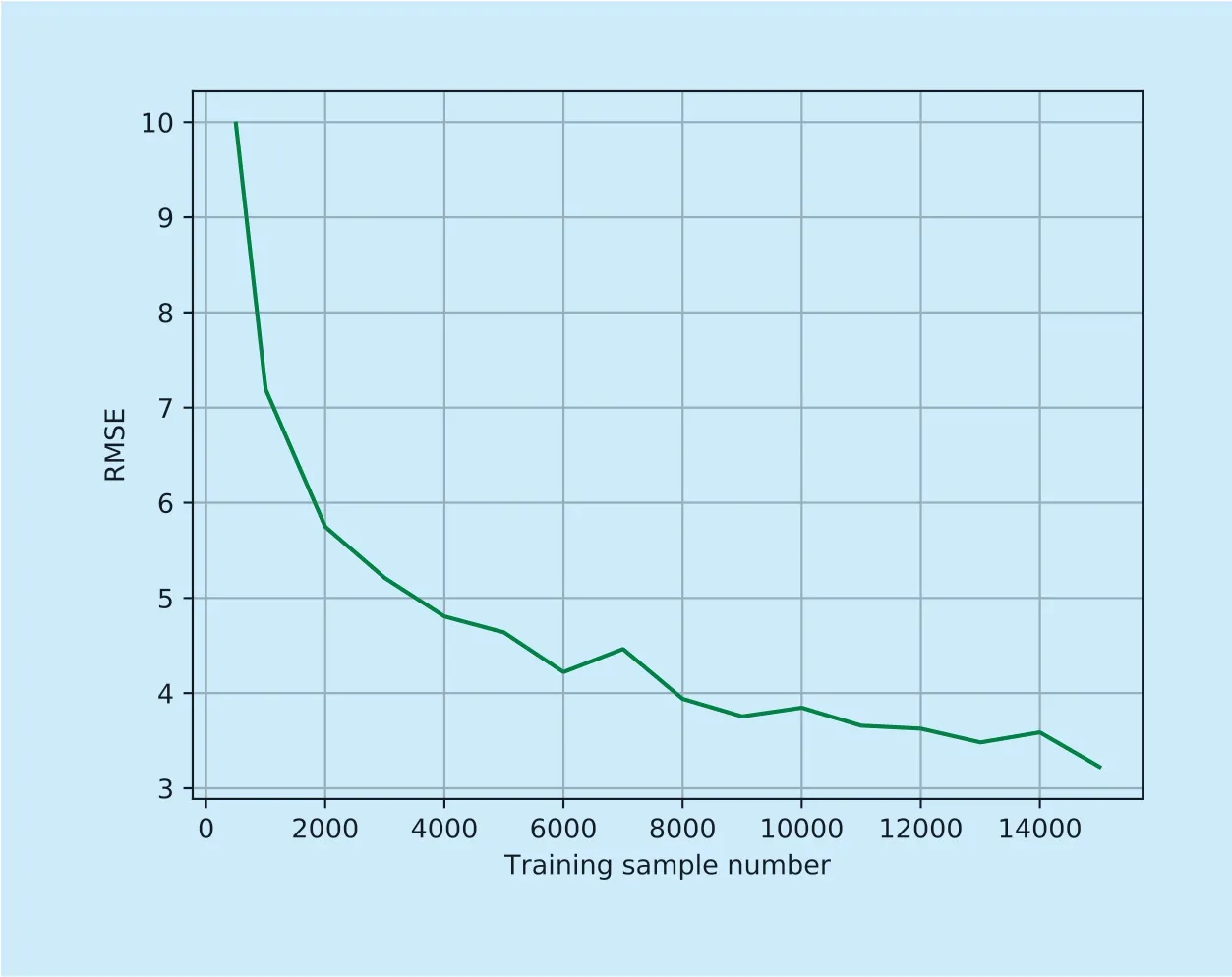
Fig.7.RMSEvary with number of training samples.

3)Influence by number of training samples

In research [22],10 million training samples are generated using finite difference method (FDM).In our experiment,15000 one-second clips are generated using FEM for training.In general,the network needs training samples as many as possible.However,it is not practical to collect too many training samples.Therefore,the results are tested on different number of training samples.RMSE varying with number of training samples is given in figure 7.It is observed that the RMSE decreases along with the increasing of training sample number.Moreover,the decent degree becomes slower with the increase of training samples.In practice,if the precision requirements are not so strict,the request for training data number is tolerable.

V.CONCLUSION

Source localization of EEG signal is still a challenging and promising task.To solve the EEG inverse problem,the key point is to find the function between the source signal and measured sEEG signal.Traditional methods solve the problem with assumptions of some priori knowledge,which could be restrict.Moreover,many other methods learn the function between source and sEEG signal from data without considering the coupled spatio-temporal information.The development of deep learning algorithms provides a good way to learn the function between source and sEEG signal with large amount of data.This work presents a novel method to localize the source signal with sequence to sequence LSTM network which learn the spatio-temporal information from training samples.With experiments on simulated data,the localization error distance of the proposed method is less than 5 mm.Moreover,the proposed method shows better robustness to noise.By comparing the network with fully connected network and single layer LSTM,the proposed network performs excellently with better results and relatively few trainable parameters.If the data for training is generated from forward problem,the learned network is equivalent to solving the inverse problem.However,if the EEG generation can be modeled using more complicated method to make them closer to real situation,source locating problem can be solving by learning the samples without calculating the inverse process.

If the data for training is large enough and real,the learned relation may be independent of head model and conduction model resulting in prediction that is more accurate.In conclusion,solving the EEG inverse problem with artificial neural network is still a promising and challenging research field.In the future,we will focus our attention on generating source imaging with deep neural network to try to solve the multi-source problem.We will try to modify the structure of spatio-temporal network to better resolve EEG source localization.

ACKNOWLEDGMENT

This work was supported by the National Natural Science Foundation of China (No.61672070,61501007,11675199,61572004 and 81501155),the Key Project of Beijing Municipal Education Commission (No.KZ201910005008),general project of science and technology project of Beijing Municipal Education Commission (No.KM201610005023),the Beijing Municipal Natural Science Foundation (No.4182005),Clinical Technology Innovation Program of Beijing Municipal Administration of Hospitals (No.XMLX201805) and Beijing Municipal Science ＆ Tech Commission (No.Z171100000117004).