The General Conjugate Gradient Method for Solving the Linear Equations
2019-07-18 09:08:20FangXimingLingFengFuShouzhong
数学理论与应用 2019年2期
Fang Ximing Ling Feng Fu Shouzhong
(School of Mathematics and Statistics, Zhaoqing University, Zhaoqing 526000, China)
Abstract In this paper, by introducing a nonsingular symmetric parameter matrix, we present the general conjugate gradient(GCG) method based on the conjugate direction method, which extends the conjugate gradient(CG) method and differs from the preconditioned conjugate gradient(PCG) method. The numerical experiments are performed to show the effectiveness of this method.
Key words Symmetric positive definite matrix Conjugate gradient method Iterative method
1 Introduction
Consider a real linear equations
Ax=b,
(1.1)
whereA∈Rn×nis a symmetric positive definite matrix andb∈Rn. WhenAis a large and sparse matrix, we often apply the iterative methods to solve it, see [1-7]. Some popular iterative methods, for instance, the Jacobi method, the Gauss-Seidel(GS) method, the successive overrelaxation(SOR) method, the generalized minimal residual(GMRES) method, the conjugate gradient(CG) method, the preconditioned conjugate gradient(PCG) method, and other iterative methods can refer to [7-12] and the references therein.
The CG method is a very popular iterative method for solving (1.1). In theory, the CG method can find out the true solution innsteps. In practice, we usually carry less thannsteps and obtain an approximate solution especially for the large and ill-posed problems. In the solving process, the conjugate vectorpkis needed in each step. In order to producepk, both the residualrkand the prior conjugate vectorpk-1are indispensable. In this paper, we use the general conjugate vectors ofAto construct the solution of (1.1). By introducing a nonsingular symmetric parameter matrixP, we applyp1,pk-1andPrk-1to generate the next conjugate vectorpkofA. Then the approximate solution can be represented by the former approximate solution and the conjugate vectorspk. In this way, we present the general conjugate gradient(GCG) method, which is different from the CG method and PCG method.
This paper is organized as follows. We introduce some preliminary knowledge about the conjugate direction method for solving the linear equations in Section 2. Then we propose the general conjugate gradient method in Section 3 and the algorithm in Section 4, respectively. Some numerical experiments are given and discussed in Section 5. Finally, we end this paper by some conclusion remarks in Section 6.
2 Preliminaries
In this section, we give some preliminary knowledge about the conjugate direction method for solving (1.1).
Letx*=A-1bbe the true solution of (1.1), which satisfies
(2.1)

(2.2)
According to the uniqueness of the coordinates, combining with (2.1), if we set
x1-x0=α1p1∈span{p1},
…
…
(2.3)
that is,xkapproaches to the true solutionx*of (1.1) gradually by the way
x1-x0,x2-x0,…,xk-x0,…,xn-1-x0,xn-x0=x*-x0,
(2.4)
then we have
(2.5)

rk-1=b-Axk-1,
(2.6)
then another calculation formula ofαkcan be obtained as follows:
(2.7)
Thus, from (2.2) and (2.7) we have
(2.8)
So, once we obtain the approximate solutionxk-1and theAconjugate vectorpk, we can calculateαkfrom (2.8) and then construct the next approximate solutionxkof (1.1) by (2.3), fork=2,3,….
3 The general conjugate gradient method

For a positive definite symmetric matrixA, it is difficult to obtain allnconjugate vectors at the same time. We construct theAconjugate vectorpk-1gradually through adding new independent vector one by one. Set an arbitrary vectorp1≠0 to be the firstAconjugate vector, and suppose that we have theAconjugate vectorsp1,p2,…,pk-1, then the follow-upAconjugate vectorpkshould satisfy the following relation expression
(3.1)
Suppose
(3.2)
andp1≠0. HerePis a given nonsingular symmetric matrix andγk-1≠0 is a real undetermined parameter.

(3.3)
So
(3.4)
In addition, from (2.5) we can obtain
(3.5)
(3.6)
From (2.3) and (3.2), applying mathematics induction method, it is easy to prove the following relations.
span{p1,p2,…,pk}=span{p1,Pr1,…,Prk-1},k=2,3,….
(3.7)
So, from (3.6) and (3.7), we have
rk-1⊥span{p1,p2,…,ps}=span{p1,Pr1,…,Prs-1},s≤k-1,k≥2.
(3.8)
Similarly, from (2.3), we have the following three expressions
xs-xs-1=αsps∈span{ps},s=1,2,…,
rs-rs-1=-αsAps,s=1,2,…,
(3.9)

(3.10)
Then, we obtain the very simple calculating formula ofpkin (3.2) whenαs≠0, that is
(3.11)

From (3.10), we can find thatβkandγkhave the multiple relationship. Then we can letγkbe a nonzero constant, such asγk≡1 for convenience.
In a word, if we select a real nonsingular symmetric matrixPand an initial vectorx0with an arbitrary conjugate vectorp1≠0, then from (2.7),αk,βk,pkandxkcan be generated gradually from (3.10), (3.11), (2,3), (2.8) and (3.4).
All above can be summarized as follows
xk-1=xk-2+αk-1pk-1,
rk-1=b-Axk-1,
(3.12)
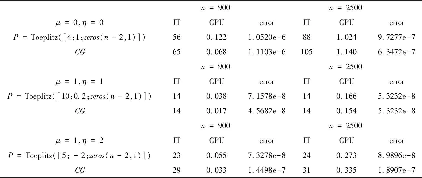
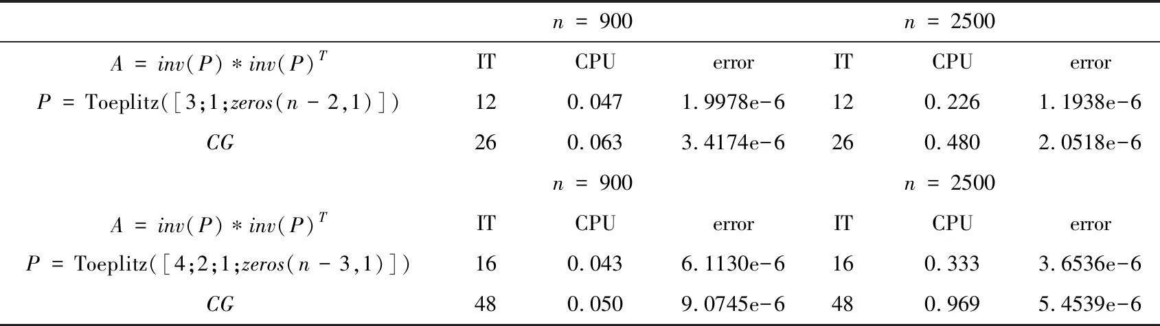
Remark 3.1The above derivations are based on the situationrk≠0,k= 1,2,…. If some residualrs-1=0, it is apparent that the true solutionx*=xs-1. Then from (3.10) and (3.12), we haveps=0, which is already not theAconjugate vector. Ifps=0,s Now, we obtain a method for solving (1.1), that is (3.12), which is called the general conjugate gradient (GCG) method and belongs to the conjugate direction method in nature. The main character of this method is that the residual vectors are applied and a real nonsingular symmetric matrix is introduced. The conjugate vectors can be obtained in a simple way. For the GCG method, the following conclusion can be proved easily from the above construction process ofpkand the derivative process ofxk. Theorem 3.1Suppose for a given initial vectorx0, the general conjugate gradient method (3.12) carriesm( (3.13) 4) span{p1,p2…,pk}=span{p1,Pr1,…,Prk-1}. ProofFrom (3.6), the conclusion 1) holds; from (3.8), the conclusion 2) holds; from (3.1), the conclusion 3) holds; and from(3.7), the conclusion 4) holds. In this section, we present the algorithm of the general conjugate gradient (GCG) method (3.12) as follows. Algorithm 1 The GCG methodInput: Input A,b,P,x0,p1,σ,k=3,n=length(b)>3.Output: xk,δ,k.1: Compute α1,x1,r1,β1,δ=norm(r1) based on (3.12).2: Compute p2.3: while k In this section, we compare the general conjugate gradient(GCG) method with the conjugate gradient(CG) method by the numerical examples. Example 1Let the coefficient matrixA∈Rn×nin (1.1) be with S=tridiag(-1,4,-1)∈Rm×m is a tridiagonal matrix. B=tridiag(1,0,1)∈Rn×n. Table 1 The comparison between GCG and CG From Table 1, we can find that the parameter matrixPhas some influence on the GCG method. If we select an appropriatePand combine with the fast algorithm about multiplication of matrix and vector, it is possible to decrease the iteration steps while deceasing the running time. Compared with the CG method, whenn=900, the GCG method with a symmetric positive definite Toeplitz matrixPhas no superiority, though the iteration steps are smaller under the same stop iteration criterion. However, whenn=2500, the result is different, the GCG method is better than the CG method in both the iteration steps and the running time. Example 2Let the coefficient matrixAin (1.1) beA=inv(P)*inv(P)T, wherePis just the nonsingular symmetric parameter matrix in the GCG method. Set the true solutionx*, the generated way ofb,x0,p1, the value ofγk-1, the stopping iteration criterionσand the calculation way oferrorto be the same as those in Example 1. The numerical results are shown in Table 2 as follows, where the symbol Toeplitz(α) denotes the symmetric Toeplitz matrix withαbeing the first column. Table 2 The comparison between GCG and CG From Table 2, we can find that the superiority of the GCG method is more obvious. Both the iteration steps and the running time are decreased greatly compared with the CG method under the same iteration condition. In this paper, we present the general conjugate gradient (GCG) method based on the conjugate direction method by introducing a nonsingular symmetric matrix and applying the residual vector with the former conjugate vector and the first conjugate vector to construct the next conjugate vector. The numerical results show that the GCG method is effective sometimes.
4 Algorithm


5 Numerical experiments


6 Conclusion remarks