Optimization of Well Position and Sampling Frequency for Groundwater Monitoring and Inverse Identification of Contamination Source Conditions Using Bayes’ Theorem
Shuangsheng Zhang , Hanhu Liu Jing Qiang , Hongze Gao , Diego Galar and Jing Lin
Abstract: Coupling Bayes’ Theorem with a two-dimensional (2D) groundwater solute advection-diffusion transport equation allows an inverse model to be established to identify a set of contamination source parameters including source intensity (M), release location (0X,0Y) and release time (0T), based on monitoring well data.To address the issues of insufficient monitoring wells or weak correlation between monitoring data and model parameters, a monitoring well design optimization approach was developed based on the Bayesian formula and information entropy.To demonstrate how the model works, an exemplar problem with an instantaneous release of a contaminant in a confined groundwater aquifer was employed.The information entropy of the model parameters posterior distribution was used as a criterion to evaluate the monitoring data quantity index.The optimal monitoring well position and monitoring frequency were solved by the two-step Monte Carlo method and differential evolution algorithm given a known well monitoring locations and monitoring events.Based on the optimized monitoring well position and sampling frequency, the contamination source was identified by an improved Metropolis algorithm using the Latin hypercube sampling approach.The case study results show that the following parameters were obtained: 1) the optimal monitoring well position (D) is at (445, 200); and 2) the optimal monitoring frequency (Δt) is 7, providing that the monitoring events is set as 5 times.Employing the optimized monitoring well position and frequency, the mean errors of inverse modeling results in source parameters were 9.20%, 0.25%, 0.0061%, and 0.33%, respectively.The optimized monitoring well position and sampling frequency can effectively safeguard the inverse modeling results in identifying the contamination source parameters.It was also learnt that the improved Metropolis-Hastings algorithm (a Markov chain Monte Carlo method) can make the inverse modeling result independent of the initial sampling points and achieves an overall optimization, which significantly improved the accuracy and numerical stability of the inverse modeling results.
Keywords: Contamination source identification, monitoring well optimization, Bayes’ Theorem, information entropy, differential evolution algorithm, Metropolis Hastings algorithm, Latin hypercube sampling.
1 Introduction
Sudden releases of contaminants to groundwater occur from time to time, which pose a serious threat to human health and can damage the environment.However, the source release locations, times, source strength and intensity are often unknown partially due to the detections of contaminants in groundwater come long after the release occurrences.Therefore, a better evaluation of source conditions is of great and practical significance to the remediation of groundwater contamination.
Using a groundwater flow and solute transport model to back-estimate the potential source conditions is here referred as contamination source inverse identification.Essentially, it is to use groundwater monitoring data to back-calculate the model input parameters (or to define the source conditions).A number of researchers employed the Bayes’ Theorem solving inverse problems, such as, Sohn et al.[Sohn, Small and Pantazidou (2000)]; Zeng et al.[Zeng, Shi, Zhang et al.(2012)]; Chen et al.[Chen, Izady, Abdalla et al.(2018)].Other methods solving inverse problems include geostatistics method [Snodgrass and Kitanidis (1997); Lin, Le, O’Malley et al.(2017)]; differential evolution algorithm [Ruzek and Kvasnicka (2001); Ramli, Bouchekara and Alghamdi (2018); Zhao (2007)]; genetic algorithm [Giacobbo, Marseguerra and Zio (2002); Mahinthakumar and Sayeed (2005); Bahrami, Ardejani and Baafi (2016); Bozorg-Haddad, Athari, Fallah-Mehdipour et al.(2018)]; the simulated annealing algorithm [Dougherty and Marryott (1991); Marryott, Dougherty and Stollar (1993)], and so on.Those above can be divided into deterministic methods and nondeterministic methods.Among the nondeterministic methods, the Bayesian statistical method uses the monitoring data to adjust the model input parameter, and then combines the sets of parameters prior probability density function with the sample likelihood function, so that forming a statistical method that is very flexible, intuitive, robust and easy to understand.This is why the Bayesian statistical method or Bayes’ Theorem has become extensively employed in engineering applications.
Using the Bayesian statistical approach to reversely identify the model parameters (or the source conditions in this study), it is often necessary to solve the posterior estimation value or posterior distribution of the parameters.When the parameter dimension is not particularly high, a numerical integral method or normal approximation method can be used to solve the posterior estimation value or posterior distribution of the parameters [Tanner (1996)].However, with the increase of the parameter dimension, the computational complexity of the numerical integral method will increase exponentially, which results in the difficulty of the solution process.So, the Monte Carlo Method [Roberts and Casella (2004)] with independent samplings as an approximate solution is often used to solve the question.The Markov chain Monte Carlo method, as an efficient and rapid sampling method, has been widely used such as by Metropolis et al.[Metropolis, Rosenbluth, Rosenbluth et al.(1953)]; Hastings [Hastings (1970)]; Haario et al.[Haario, Saksman and Tamminen (2001)]; Xu et al.[Xu, Jiang, Yan et al.(2018)].
In real engineering applications, it is impractical to obtain a desired number of monitoring wells and samples due to the limitations of funds and/or restrictions of site conditions.Therefore, in reality, there is always insufficient data available to use, which could potentially result in ill-posed characteristic of inverse problem [Carrera and Neuman (1986)].Therefore, to address the above limitations, the monitoring well locations together with the sampling frequency need to be optimized to potential satisfy the inverse parameters evaluation requirements.To do so, a few steps should follow.First, the data for monitoring plan need to be quantified by setting up an objective function [Zhang (2017)], of which the most commonly selected objective function is signal-to-noise ratio (SNR) [Czanner, Sarma, Eden et al.(2008)], i.e., the relative entropy from the Bayesian formula [Huan and Marzouk (2013); Zhang (2017); Lindley (1956)].The SNR and relative entropy are applicable to nonlinearity models with an assumption that the parameter distribution is non-Gaussian [Huan and Marzouk (2013); Lindley (1956)].Groundwater flow and transport models are mostly nonlinear so that the SNR approach and Bayesian formula using relative entropy apply.However, the SNR approach only factor in the effect of monitoring errors on the monitoring data, while the relative entropy does not include the influence of the prior distribution of parameters on the posterior distribution.To overcome the limitations of both the SNR approach and the relative entropy approach, the information entropy by Shannon [Shannon (1948)] was employed since it measures of information uncertainty.The greater of the information uncertainty, the greater of the information entropy will be.The information entropy in the posterior distribution of model parameters is used as a measurable value of the monitoring data.The smaller of the information entropy, the smaller of the uncertainty of the model parameters will be, and the better of the parameter inverse estimation results will expect.
This paper provides an example problem with an instantaneous release of a contaminant in a confined groundwater aquifer.The information entropy of the posterior distribution of the model parameters based on the Bayesian formula was used as the measurement value of the monitoring data.And the optimization of the monitoring well position and sampling frequency was solved by the Monte Carlo method and a differential evolution algorithm under the condition of single well monitoring and determining monitoring times.Relying on the optimized monitoring well program, the contamination source is identified by an improved Metropolis algorithm based on Latin hypercube sampling.This paper could provide reference for the optimization design of groundwater contamination monitoring wells and inverse problem of contamination source identification.
2 Study methods
2.1 Parameter inversion based on bayesian formula
The Bayesian formula [Berger (1995)] is expressed as follows:

Where,
·α is the unknown model parameter;
·d is the monitoring data;
Assuming that
·The number of the unknown parameters in the model are m, namely
·the environmental hydraulic model parameters are all distributed in a specific range;
·each parameter obeys uniform distribution;
So, the prior probability density function of model parameteriα can be defined as:

And the total prior distribution p(α)can be expressed as:

Assuming that the number of monitoring values in the model are n, namelyWhere diindicates the ithmonitoring value.indicates the corresponding ithpredictive value.Thenindicates the measurement error, i =1,2,,n .Assuming that εiobeys normal distribution with mean μ=0; and standard deviation σ=0.05; and eachiε is mutually independent, so the conditional probability density functioncan be expressed as follows:

Combining the above functions (1), (2), (3) and (4), the posterior probability density functionof α can be expressed as follows:


Eq.(6) can be viewed as a function about parameters α under the condition that the measured value is fixed.Since it is difficult to draw the explicit expression of Eq.(6) by a numerical integral method, the Markov Chain Monte Carlo method is employed to solve the equation.
The core of Markov Chain Monte Carlo method is Monte Carlo simulation method and Markov chain sampling method.When the sample points are sufficient as “probability events”, the probability can be approximately represented as frequency, which is the essence of the Monte Carlo simulation method.Employing the Markov chain sampling method can ensure that the Markov chain select more data points in the area with high probability, which can save the workload of the Monte Carlo simulation.The Metropolis algorithm is a classic Markov Chain Monte Carlo method, and therefore widely used.The Metropolis algorithm is utilized to find the solution in this article.The details of the Metropolis algorithm can be found in literature [Metropolis, Rosenbluth, Rosenbluth et al.(1953); Hastings (1970)].
2.2 Monitoring well design optimization
The optimization of the monitoring plan mainly includes monitoring well quantity, position and monitoring frequency.As an example, a single well is used to illustrate the general approach:
Assuming that the monitoring well position isD, from which the monitoring data is still recorded as d.Then the Bayesian formula can be rewritten as:

Since the prior distributionparameter α suggests a preliminary set of unknown parameters (that is not affected by the monitoring well position, namely(7) becomes the following:

Normalizing the integral constantresults in the probability of monitoring data d at position D expressed asin the following format:

Assuming that the probability density is a function of a random variableX [expressed as f(x)], the information entropy of X in the interval [a,b] can be defined as follows [Shannon (1948)]:

So we can use the monitoring data d at position D to back-calculate the unknown parameterα, and then the posterior probability density functioncan be obtained.The information entropy of the posterior distribution α can be similarly expressed as:

The left side of Eq.(11) contains monitoring datad, which can be considered as a random variable, with a probability density functionIn order to obtain a function only containing variable D, both sides of Eq.(11) are multiplied byThen the expectationof the information entropycan be written as:

It is difficult to derive the explicit expression of Eq.(12).So, the Monte Carlo method [Huan and Marzouk (2013)] is used to find an approximately solution.
Using Eq.(8), Eq.(12) can be rewritten as follows:

Since the prior distribution p(α) is given by Eqs.(2) and (3), the information entropyin Eq.(13) can be written as Thissuggests that the greater of information entropy is, the greater of the uncertainty of α.When p(α) remains unchanged,ln p(α)-stays the same.In order to get the minimum value of E(D),we only calculate the minimum value of
If we name U(D) as follows:
the monitoring value d in the Bayesian formula could reduce the uncertainty of parametersα, based on Lindley (1956).
Eq.(14) can be solved by Monte Carlo method as follows:

Firstly, we can randomly draw Nsamples from the prior distribution p(α) of unknown parameter α, namelySecondly, for each i∈ N, we can get a sample difrom the conditional probability density functionaccording to Eq.(4), and a total of N.Finally, each group ofis brought into Eq.(4), and we can obtain theEq.(15).From Eq.(9),Eq.(15) can be rewritten aswill be solved by the Monte Carlo method as follows:

2.3 Improved metropolis algorithm based on latin hypercube sampling
The Metropolis algorithm is a classic MCMC method, which is widely used.However, it is prone to local optimization, or difficult to converge by using Metropolis algorithm to invert the model parameters.Moreover, sampling efficiency is low.This study proposes an improved Metropolis algorithm based on Latin hypercube sampling.
2.3.1 Metropolis algorithm
The Metropolis algorithm was first proposed by Metropolis et al.[Metropolis, Rosenbluth, Rosenbluth et al.(1953)], and further revised by Hastings [Hastings (1970)].Specific steps are as follows:
(2) Make the uniform distributionas the proposal distribution, and satisfy the symmetric random walk.Here step represents the size of a random walk.Then a candidate sample Ζ*is generated fromwhile u is extracted from the uniform distribution (0,1)U randomly.
(4) Repeat Steps (2) and (3) till the given iterative times are reached.
2.3.2 Improved metropolis algorithm based on latin hypercube sampling method
In order to prevent the local optimization of the inversion results, or to generate problems that are difficult to converge, this study uses the Latin hypercube sampling method [Dai (2011)] to optimize the sampling process to ensure the randomness and uniformity of the initial points of the sample.Latin hypercube sampling is a multi-dimensional hierarchical random sampling method with good dispersion uniformity and representativeness.When we want to extract q sets of samples from the prior distribution rangesm dimensional model parameters α by Latin hypercube sampling method, the specific steps are as follows:
(1) Dividing m prior distribution rangesm dimensional model parameters into qranges, which can be recorded asm×q ranges are produced.
(2) Extracting αijfrom the rangerandomly, and total m×q numbers are produced.
The following matrix is formed:
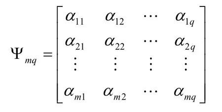
(3) Arranging the row vectorin the matrix Ψmqrandomly into a new row vectorΨmqwill be transformed into a new matrix, which is:
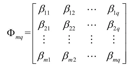
(4) Each column vector of matrix Φmqis a set of samples; and q sets of samples are combined together.
The specific steps of the improved Metropolis algorithm based on Latin hypercube sampling method are as follows:
(1) A number of q sets of initial samples are randomly obtained from the value ranges of model parameters by the Latin hypercube sampling method.
(2) Taking the q sets of samples as initial points in Step (1), q Markov Chains are generated by the Metropolis algorithm.
(3) The averages of the calculated results of q Markov Chains are taken as the final results.
The improvement of this method lies in reducing the influence of the initial point values on the result by the Metropolis algorithm as much as possible, which accords with the idea of the Monte Carlo method.
2.3.3 Convergence judgment of the improved multi-chain metropolis algorithm
In this study, the convergence of the last 50% sampling process by the multi-chain Metropolis algorithm is guided by the Gelman-Rubin convergence diagnosis method [Gelman and Rubin (1992)].The convergence indicator is as follows:

where,
·g is half the length of the Markov chain length in the multi-chain Metropolis algorithm;
·q is the number of Markov chains used for the judgment;
·Biis the variance of the means of the last 50% samples in the q Markov chains of the ithparameter;
·Wiis the average of the variance of the last 50% samples in the q Markov chains of theparameter.
3 Example application
3.1 Example overview
In a homogeneous and confined aquifer, the (2D) groundwater solute advection-diffusion equation [Zheng and Gordon (2009)] can be expressed as:

where,
·Cis the concentration of a contaminant at the monitoring position(,)xyfor the time t,(mg/L);
·t is the elapsed time from the release time (day);
·uis an average groundwater flow velocity (m/day).
The analytical solution to Eq.(18) for the instantaneous release of a contaminant at a position can be expressed as:
where,
·M is the source release intensity (g);
·h is the thickness of the aquifer (m);
·x and y are the vertical and horizontal distances from the contamination source (m), respectively;
·k is the effective porosity of the aquifer.
Providing that the aquifer is homogeneous with a coordinate system in 2D as shown on Fig.1; the release location of a contaminant is in the region of S; groundwater flow direction follows the x-axis; and the monitoring well position isD; the regional hydrogeological parameters are presented in Tab.1.

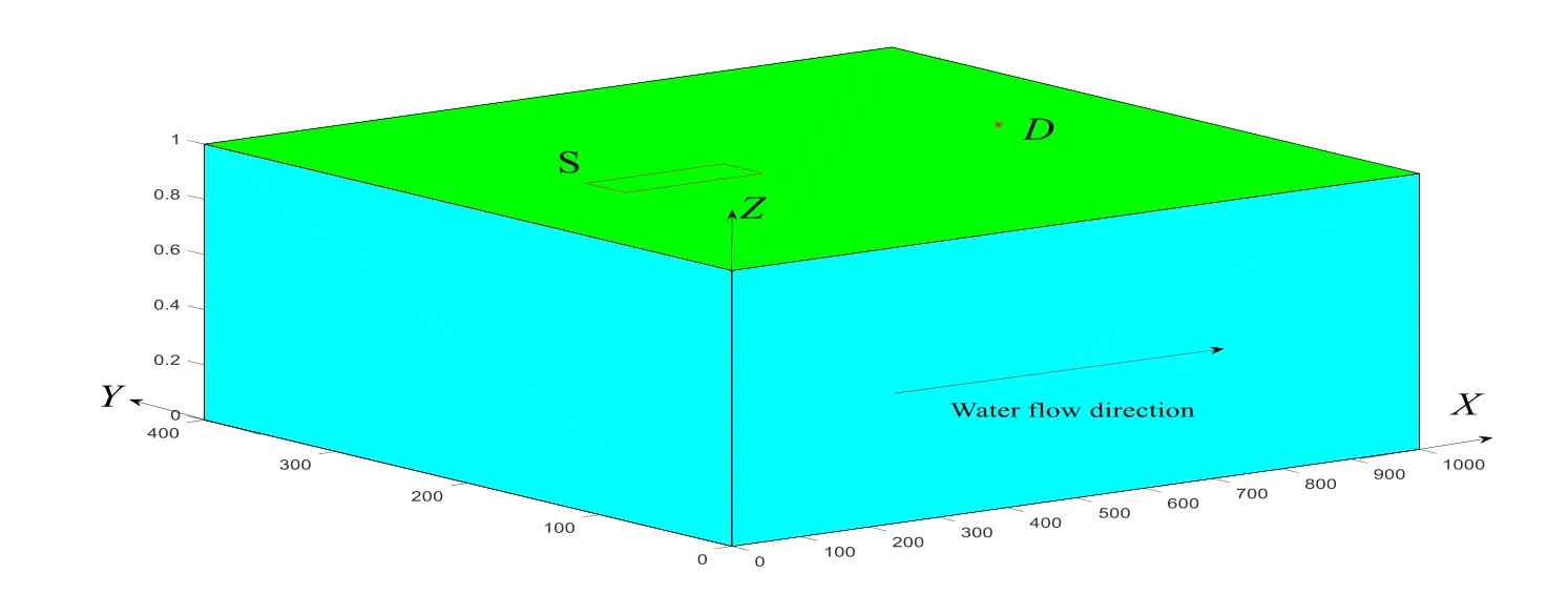
Figure 1: Schematic diagram of the example problem

Table1: Known hydrological parameters in the studied area

Table 2: Value range of parameter α to be solved in the studied area
3.2 Monitoring well position optimization
A certain moment without pollution discharged in S is taken as the initial time, at this time t=0.The prior distribution ranges of the parameters to be solved in the studied area are shown in Tab.2.The monitoring duration starts from t=70 and ends at t=90.A monitoring time interval is 4 days.Providing the solute migration velocity is 5 m/day, the possible range of optimal monitoring well position D*is within this range:
The optimization problem of monitoring well position can be generalized as follows:

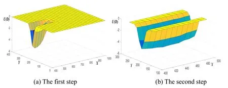
Figure 2: Three dimensional stereograms of the two-step Monte Carlo method to solve U(D)
In order to verify the effectiveness of the monitoring well design optimization using the Bayesian formula, the information entropy E(D) and the relative root mean square error of inversion results RT(D) are used as an evaluation to compare the results of using 8 monitoring well positions randomly selected inwith this settings for*D
(1) Information Entropy E(D):The coordinates of the 8 monitoring wells are shown in Tab.3.From Eqs.(13), (15), (16), U(D) and E(D) of the above 8 monitoring wells,*D can be solved in Tab.3.As illustrated in Tab.3, the information entropy at*D= (445,200) is the smallest.
(2) Relative Root Mean Square Error of Inversion Results RT(D):the relative root mean square error between the posterior mean estimate MDiand real parameterR, which demonstrates the comprehensive influence of Dion the inversion results.20 sets of parameters are randomly and evenly obtained from the prior distribution of parameterα as the real values (Tab.4).Corresponding to the 8 monitoring positions in Tab.3, 160 sets of monitoring values with measurement error ε can be calculated using Eq.(18).Then the parameterα can be inversely estimated using the generated monitoring values (with a length of the Markov chain of 25,000).In order to ensure the accuracy of inversion results, only the last 2,000 samples after a stabilization trend are used to calculate the posterior mean value MDi.Then applying theand R in Tab.4 to Eq.(20) as follows:

Where,
·j is the jthset of parameterα;
·k is the kthcomponent of parameterα.
Table 3: and of 8 monitoring wells

Table 3: and of 8 monitoring wells
i 1 2 3 4 5 6 7 8 D (445,200) (657,248) (470,184) (590,191) (550,200) (420,190) (460,195) (406,180) i UD -4.5369 -4.92*10-3 -2.3546 -0.7079 -2.2596 -3.2233 -4.2440 -1.2195 ( )( )i ED 13.8430 18.3749 16.0253 17.6720 16.1203 15.1556 14.1359 17.1604 ( )i RTD i 0.1550 0.1880 0.1787 0.1833 0.1764 0.1575 0.1580 0.1744
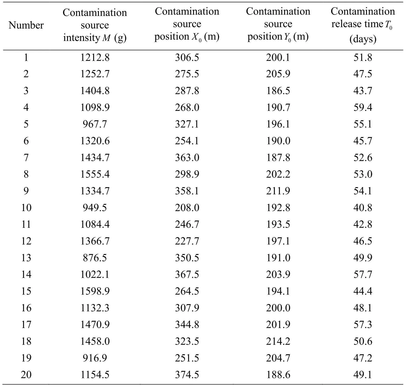
Table 4: 20 sets of real parameters obtained from the prior distribution
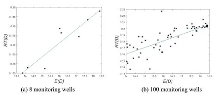
Figure 3: The fitting diagram of the relationship between E(D) and RT(D)
3.3 Monitoring frequency optimization
Assuming that monitoring well position has been determined, with,which is the best estimated monitoring position.The monitoring count is set as 5 times, and the first monitoring time is set as 70t=.The monitoring interval (tΔ) is defined as a time interval between 2 monitoring time with only an integer value.The information entropy of posterior distribution of parameterα under a monitoring interval can be expressed asand thereforeThe different monitoring intervals are expressed asThe calculation methods ofandare the same as that of E(D) and RT(D) in Section 3.2.The calculation results are shown in Tab.5.It can be seen from Tab.5 that bothandreach minimum values when Δt=7.The optimal monitoring frequency is obtained to be 7 at the optimized monitoring well position
Table 5: and of 12 monitoring cycles
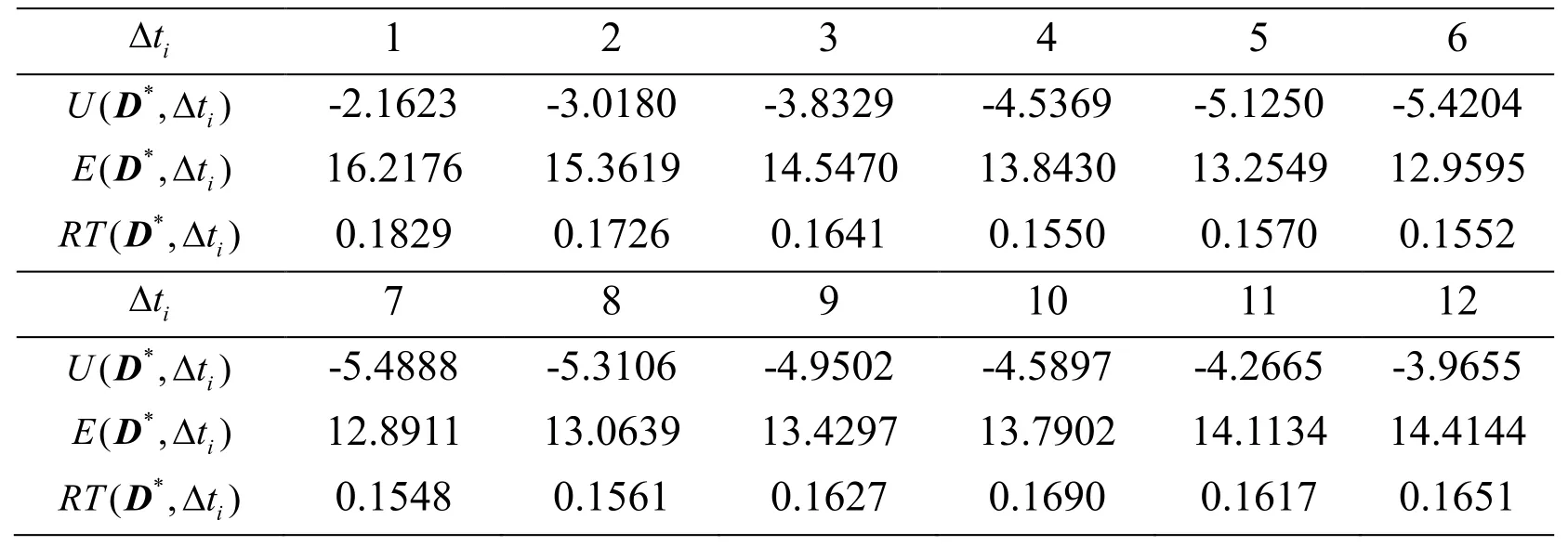
Table 5: and of 12 monitoring cycles
Δ 1 2 3 4 5 6 t i*U tΔD -2.1623 -3.0180 -3.8329 -4.5369 -5.1250 -5.4204 (,)i*E tΔD 16.2176 15.3619 14.5470 13.8430 13.2549 12.9595 (,)i*RT tΔD 0.1829 0.1726 0.1641 0.1550 0.1570 0.1552 (,)i Δ 7 8 9 10 11 12 t i*U tΔD -5.4888 -5.3106 -4.9502 -4.5897 -4.2665 -3.9655 (,)i*E tΔD 12.8911 13.0639 13.4297 13.7902 14.1134 14.4144 (,)i*RT tΔD 0.1548 0.1561 0.1627 0.1690 0.1617 0.1651 (,)i
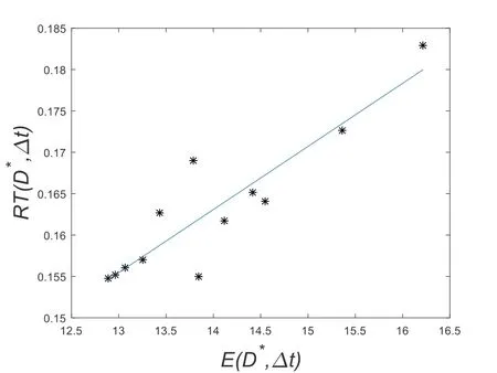
Figure 4: The fitting diagram of the relationship between and
3.4 Contamination source identification based on the optimized monitoring plan
From Sections 3.2 and 3.3, we know that the optimal monitoring well plan for the example in this paper is that monitoring well positionand monitoring frequency is 7.
3.4.1 Solution results by the metropolis algorithm
In this section, the model parameters are solved by adopting the classic Metropolis algorithm to build the Markov chains.However, the iterative curves of the 4 parametersto be estimated vary widely because of the different initial sample points by the Markov chains.Taking M as an example, different initial sample,such as an initial sample Set 1 ofand a sample Set 2 ofare randomly selected,the iterative curves are produced as shown on Fig.5(a) and Fig.5(b).
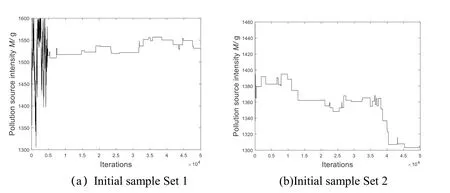
Figure 5: Iterative curves of model parameter M based on the Metropolis algorithm with different initial samples
It can be seen from Fig.5(a) that when the initial sample point is M1=1500.1 g and the Metropolis algorithm is iterated to 5000 times, the parameter M value gradually becomes stable, and eventually converges to M≈1520g.However, the value is quite different from the true value (M=1212.8 g), with an error of 25.3%.Fig.5(b) shows that when the initial sample point is M1=1449.4 g and the iteration reache 50,000 times, the parameter M value still does not converge.Therefore, when the classical Metropolis algorithm is used to solve the contamination source intensity, the solution result is greatly affected by the initial sample point.This suggests that it is prone to local optimum or difficult to converge.What’s more, it is speculated that similar problems may occur to another 3 parameters
3.4.2 Solution results by the improved multi-chain metropolis algorithm
Giving that the solution results of the Metropolis algorithm are affected by the initial sample points, the improved multi-chain Metropolis algorithm is used to solve the same problem.The posterior probability histograms of the contamination source parameters are drawn by the improved multi-chain Metropolis algorithm, as shown on Fig.6 (where the red line shows the true value).
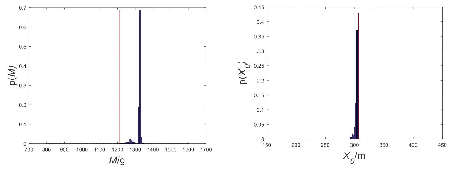
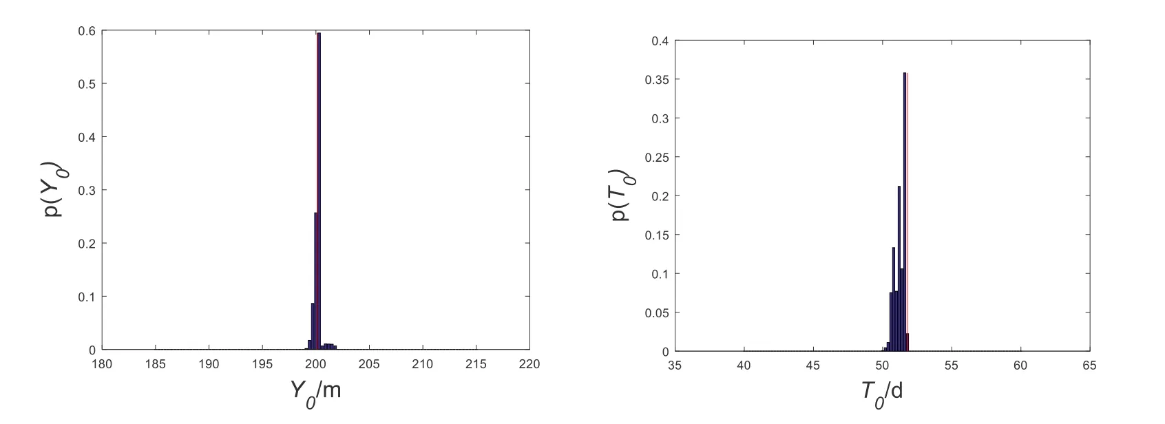
Figure 6: Posterior probability histograms of model parameters based on improved Metropolis algorithm
In the inversion process, each Markov chain has a length of 50,000 for a total of 40 chains.When the evolutionary generations of the parallel Markov chains reach 40,000, the convergence judgment index of 4 parameters are asAt this time, the Markov chains of all parameters have converged.Then the previous unstable 40,000 Markov chains results are excluded, so that only the last 10,000 stable results are used to perform the posterior statistical analysis.The results are shown in Tab.6.From Tab.6, it can be seen that the Metropolis algorithm based on the Latin hypercube sampling method can achieve overall optimization in inversion results and can effectively improve the accuracy of inversion results.

Table 6: Posterior statistical results of model parameters based on improved Metropolis algorithm
3.4.3 Influence of prior distribution range on the parameter inversion results
Taking the parameter M as an example, 10 sets of parameters prior distribution ranges (as shown in Tab.7) are selected to verify the influence of the prior distribution range on the parameter inversion results.All of the observations are observed through the optimal observation scheme.different prior distribution ranges are calculated in the process as in Section 3.2.The values are shown in Tab.8, and the linear fit betweenon Fig.7.
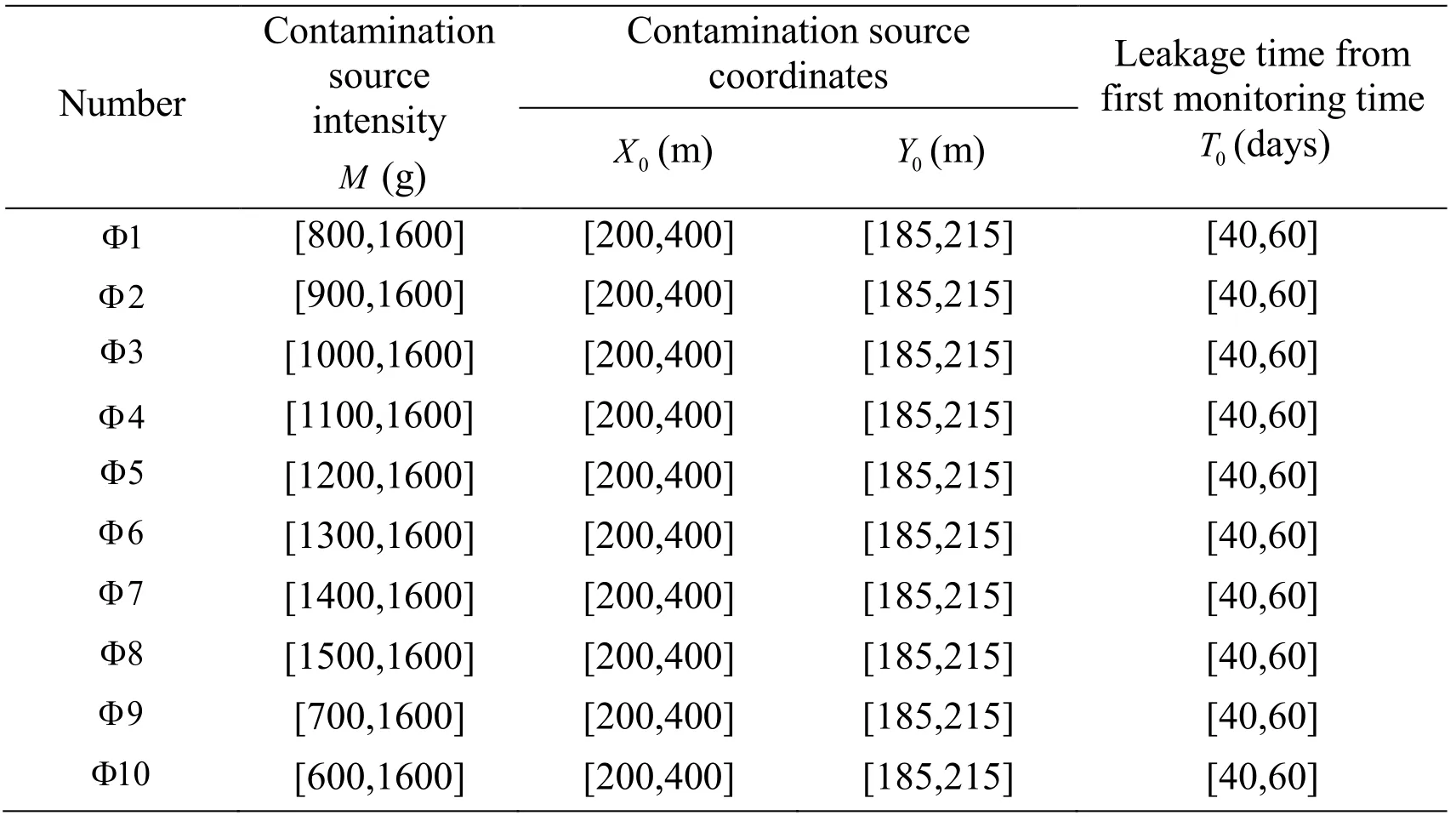
Table 7: 10 sets of parameters prior distribution ranges
Table 8: different parameters prior distribution ranges
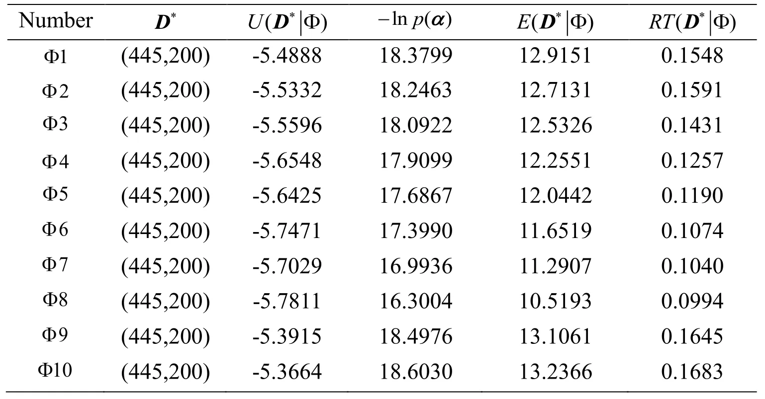
Table 8: different parameters prior distribution ranges
Number *D - α ln ()pRT *ΦD( )1Φ (445,200) -5.4888 18.3799 12.9151 0.1548 Φ (445,200) -5.5332 18.2463 12.7131 0.1591 3 2 Φ (445,200) -5.5596 18.0922 12.5326 0.1431 4 Φ (445,200) -5.6548 17.9099 12.2551 0.1257 5 Φ (445,200) -5.6425 17.6867 12.0442 0.1190 6 Φ (445,200) -5.7471 17.3990 11.6519 0.1074 7 Φ (445,200) -5.7029 16.9936 11.2907 0.1040 8 Φ (445,200) -5.7811 16.3004 10.5193 0.0994 9 Φ (445,200) -5.3915 18.4976 13.1061 0.1645 10 Φ (445,200) -5.3664 18.6030 13.2366 0.1683
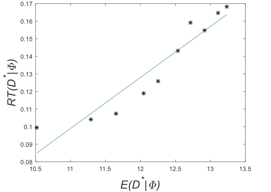
Figure 7: The fitting diagram of the relationship between
In Tab.6, the parameters X0,Y0,T0have better inversion results since the mean errors are all less than 0.5%.However, the inversion mean error of M is as high as 9.20%.It is largely because that the prior distribution range of M is larger than that of X0,Y0and T0according to the above theory.Therefore, in order to improve the accuracy of the inversion results, the prior distribution ranges of parameters should be minimized through good field investigation or experiment.
4 Conclusion
(a) Using the Bayesian formula to solve the inverse problem of contamination source identification could effectively avoid the loss of “truth values” comparing with that in the deterministic model solution process, which could improve the reliability in identifying the contamination source information (i.e., the contamination source intensity, position and release time).
(b) Both the relative root mean square error of inversion results and the information entropy of posterior distribution of parameters show a good positive linear relationship, suggesting that the information entropy can be seen as a potent indicator for inversion results.The smaller of the information entropy is, the better of the parameter inversion result will be.Therefore, the optimize design method using the Bayesian formula and information entropy can be an effective method to design a groundwater contamination monitoring well plan.
(c) The computational efficiency of the optimal design of groundwater monitoring wells could be significantly improved by coupling the two-step Monte Carlo method with the differential evolution algorithm.
(d) Utilizing the improved Metropolis algorithm based on Latin hypercube sampling to solve the inverse problem of groundwater contamination source conditions could achieve the overall optimal results with a significantly improved accuracy.And its reliability and stability are better than those of the classic Metropolis algorithm.
Acknowledgment:This work was supported by Major Science and Technology Program for Water Pollution Control and Treatment (No.2015ZX07406005), Also thanks to the National Natural Science Foundation of China (No.41430643 and No.51774270) and the National Key Research & Development Plan (No.2016YFC0501109).
References
Bahrami, S.; Ardejani, F.D.; Baafi, E.(2016): Application of artificial neural network coupled with genetic algorithm and simulated annealing to solve groundwater inflow problem to an advancing open pit mine.Journal of Hydrology, vol.526, pp.471-484.
Berger, J.O.(1995): Recent development and applications of Bayesian analysis.Proceedings 50th ISI, Book I.
Carrera, J.; Neuman, S.P.(1986): Estimation of aquifer parameters under transient and steady state conditions: 2.Uniqueness, stability, and solution algorithms.Water Resources Research, 1986, vol.22, no.2, pp.211-227.
Chen, M.J.; Izady A.; Abdalla, O.A.; Amerjeed, M.(2018): A surrogate-based sensitivity quantif ication and Bayesian inversion of a regional groundwater f low model.Journal of Hydrology, vol.557, pp.826-837.
Czanner, G.; Sarma, S.V.; Eden, U.T.; Brown, E.N.(2008): A signal-to-noise ratio estimator for generalized linear model systems.Lecture Notes in Engineering & Computer Science, vol.2171, no.1.
Dai, Y.B.(2011): Uncertainty Analysis of Vehicle Accident Reconstruction Results Based on Latin Hypercube Sampling (Ph.D.Thesis).Changsha University of Science & Technology, China.
Dougherty, D.E.; Marryott, R.A.(1991): Optimal groundwater management: 1.Simulated annealing.Water Resources Research, vol.27, no.10, pp.2493-2508.
Gelman, A.; Rubin, D.B.(1992): Inference from iterative simulation using multiple sequences.Statistical Science, no.7, pp.457-472.
Giacobbo, F.; Marseguerra, M.; Zio, E.(2002): Solving the inverse problem of parameter estimation by genetic algorithms: the case of a groundwater contaminant transport model.Annals of Nuclear Energy, vol.29, no.8, pp.967-981.
Haario, H.; Saksman, E.; Tamminen, J.(2001): An adaptive Metropolis algorithm.Bernoulli, vol.7, no.2, pp.223-242.
Bozorg-Haddad, O.; Athari, E.; Fallah-Mehdipour, E.; Loaiciga, H.A.(2018): Real-time water allocation policies calculated with bankruptcy games and genetic programing.Water Science and Techonology: Water Supply, vol.18, no.2, pp.430-449.
Hastings, W.K.(1970): Monte Carlo sampling methods using Markov chains and their applications.Biometrika, vol.57, no.1, pp.97-109.
Huan, X.; Marzouk, Y.M.(2013): Simulation-based optimal Bayesian experimental design for nonlinear systems.Journal of Computational Physics, vol.232, no.1, pp.288-317.
Lin, Y.Z.; Le, E.B.; O’Malley, D.;Vesselinov, V.V.;Tan, B.T.(2017): Large-scale inverse model analyses employing fast randomized data reduction.Water Resources Research, vol.53, no.8, pp.6784-6801.
Lindley, D.V.(1956): On a measure of the information provided by an experiment.Annals of Mathematical Statistics, vol.27, no.4, pp.986-1005.
Mahinthakumar, G.K.; Sayeed, M.(2005): Hybrid genetic algorithm-local search methods for solving groundwater source identification inverse problems.Journal of Water Resources Planning and Management, vol.131, no.1, pp.45-57.
Marryott, R.A.; Dougherty, D.E.; Stollar, R.L.(1993): Optimal groundwarter management: 2.Application of simulated annealing to a field-scale contamination site.Water Resources Research, vol.29, no.4, pp.847-860.
Metropolis, N.; Rosenbluth, A.W.; Rosenbluth, M.N.; Teller A.H; Teller E.(1953): Equation of state calculations by fast computing machines.Journal of Chemical Physics, vol.21, no.6, pp.1087-1092.
Ramli, M.A.M.; Bouchekara, H.R.E.H.; Alghamdi, A.S.(2018): Optimal sizing of PV/wind/diesel hybrid microgrid system using multi-objective self-adaptive differential evolution algorithm.Renewable Energy, vol.121, pp.400-411.
Roberts, C.P.; Casella, G.(2004): Monte Carlo Statistical Methods (Second Edition).Springer-Verlag, USA.
Ruzek, B.; Kvasnicka, M.(2001): Differential evolution algorithm in the earthquake hypocenter location.Pure and Applied Geophysics, vol.158, no.4, pp.667-693.
Sebastiani, P.; Wynn, H.P.(2000): Maximum entropy sampling and optimal Bayesian experimental design.Journal of the Royal Statistical Society, Series B (Statistical Methodology), vol.62, pp.145-157.
Shannon, C.E.(1948): A mathematical theory of communication.Bell System Technical Journal, vol.27, no.4, pp.379-423.
Snodgrass, M.F.; Kitanidis, P.K.(1997): A geostatistical approach to contaminant source identification.Water Resources Research, vol.33, no.4, pp.537-546.
Sohn, M.D.; Small, M.J.; Pantazidou, M.(2000): Reducing uncertainty in site characterization using bayes monte carlo methods.Journal of Environmental Engineering, vol.126, no.10, pp.893-902.
Tanner, M.A.(1996): Tools for Statistical Inference: Methods for the Expectation of Posterior Distribution and Likelihood Functions.Springer-Verlag, USA.
Xu, W.T.; Jiang, C.; Yan, L.; Li, L.Q.; Liu, S.N.(2018): An adaptive metropolis-hastings optimization algorithm of Bayesian estimation in non-stationary flood frequency analysis.Water Resources Management, vol.32, no.4, pp.1343-1366.
Zeng, L.Z.; Shi, L.S.; Zhang, D.X.; Wu, L.S.(2012): A sparse grid based Bayesian method for contaminant source identification.Advances in Water Resources, vol.37, pp.1-9.
Zhang, J.J.(2017): Bayesian Monitoring Design and Parameter Inversion for Groundwater Contaminant Source Identification (Ph.D.Thesis).Zhejiang University, China.
Zhang, J.J.; Zeng, L.S.; Chen C.; Chen, D.J.; Wu, L.S.(2015): Efficient Bayesian experimental design for contaminant source identification.Water Resources Research, vol.51, no.1, pp.576-598.
Zhang, J.J.; Li, W.X.; Zeng, L.Z.; Wu, L.S.(2016): An adaptive Gaussian process-based method for efficient Bayesian experimental design in groundwater contaminant source identification problems.Water Resources Research, vol.52, no.8, pp.5791-5984.
Zhao, G.(2007): Differential Evolution Algorithm with Greedy Strategy and Its Applications (Ph.D.Thesis).Harbin Institute of Technology, China.
Zheng, C.M.; Gordon, D.(2009): Applied Contaminant Transport Modeling (Second Edition).Higher Education Press, China.
 Computer Modeling In Engineering&Sciences2019年5期
- Computer Modeling In Engineering&Sciences的其它文章
- A Data-Intensive FLAC3D Computation Model: Application of Geospatial Big Data to Predict Mining Induced Subsidence
- 3D Web Reconstruction of a Fibrous Filter Using Sequential Multi-Focus Images
- Frequency Domain Filtering SAR Interferometric Phase Noise Using the Amended Matrix Pencil Model
- Monitoring Multiple Cropping Index of Henan Province, China Based on MODIS-EVI Time Series Data and Savitzky-Golay Filtering Algorithm
- Inferring Spatial Distribution Patterns in Web Maps for Land Cover Mapping
- Exploring Urban Population Forecasting and Spatial Distribution Modeling with Artificial Intelligence Technology
