On the Robustness of the xy-Zebra-Gauss-Seidel Smoother on an Anisotropic Diffusion Problem

Michely Laís de Oliveira, Marcio Augusto Villela Pinto, Simone de Fátima Tomazzoni Gonçalves and Grazielli Vassoler Rutz

Abstract: Studies of problems involving physical anisotropy are applied in sciences and engineering, for instance, when the thermal conductivity depends on the direction.In this study, the multigrid method was used in order to accelerate the convergence of the iterative methods used to solve this type of problem.The asymptotic convergence factor of the multigrid was determined empirically (computer aided) and also by employing local Fourier analysis (LFA).The mathematical model studied was the 2D anisotropic diffusion equation, in which ε>0 was the coefficient of a nisotropy.The equation was discretized by the Finite Difference Method (FDM) and Central Differencing Scheme(CDS).Correction Scheme (CS), pointwise Gauss-Seidel smoothers (Lexicographic and Red-Black ordering), and line Gauss-Seidel smoothers (Lexicographic and Zebra ordering) in x and y directions were used for building the multigrid.The best asymptotic convergence factor was obtained by the Gauss-Seidel method in the direction x for 0<ε<<1 and in the direction y for ε>>1.In this sense, an xy-zebra-GS smoother was proposed, which proved to be efficient and robust for the different anisotropy coefficients.Moreover, the convergence factors calculated empirically and by LFA are in agreement.

Keywords: Physical anisotropy, diffusion problem, finite difference method, multigrid,local Fourier analysis, Gauss-Seidel zebra.

1 Introduction

Numerical simulations on engineering application problems stand out in the research and development of technology.Computational Fluid Dynamics (CFD) is the area of scientifi c computing that studies numerical methods in order to simulate problems involving fluids in motion with or without heat exchange.

In CFD,mathematical models can be discretized by the Finite Difference Method(FDM)[Ferziger and Peric(2002)],which aims to approximate each term of the mathematical model by means of algebraic expressionsat each point of the grid,thus generating a linear system of algebraic equations,such as:

where A is the matrix of the coefficients of size N×N,T is the variable of interest,and b is the vector of independent terms,also known as source term.In order to obtain good results in CFD,it is necessary to reduce the discretization error,which implies in the use of very refi ned grids thus leading to increased computational costs.Another factor that increases CPU time(tCPU)is that the discretization of these problems results in systems of algebraic equationsin which the matrix of the coefficients have a high degree of sparsity [Burden, Faires and Burden (2016)].

In order to solve Eq.(1), direct or iterative methods, hereinafter called solvers, can be employed.As the system of algebraic equations generated is sparse and large, direct methods are not feasible due to their high computational cost [Burden, Faires and Burden (2016)].In this case, iterative methods are chosen.Such methods start from an initial guess after successive approximations and converge to a solution under certain hypotheses [Burden, Faires and Burden (2016)].

It is known that only high frequency components (oscillatory modes) of the error are reduced promptly in iterative solvers, leaving low frequency components (smooth modes) unaffected [Briggs, Henson and Mccormick (2000); Trottenberg, Oosterlee and Schuller(2001);Wesseling (2004)].Solvers that have this smoothing property are called smoothers.

The multigrid is an efficient method to accelerate the convergence rate of the smoother[Briggs, Henson and Mccormick (2000); Trottenberg, Oosterlee and Schuller (2001); Wesseling (2004); Hackbusch (2003)].It was developed with the purpose of helping iterative methods eliminate smooth components of the error.According to Trottenberg et al.[Trottenberg, Oosterlee and Schuller (2001)], smooth components in a given grid become more oscillatory in the perspective of a coarser grid.The multigrid consists of a set of grids with different degrees of refinement, which are visited during the iterative process, thus effectively reducing the entire frequency spectrum of the error.

Anisotropic problems [Wienands and Joppich (2005)] are common in engineering.In such cases, the efficiency of the multigrid method is reduced [Briggs, Henson and Mccormick (2000); Trottenberg, Oosterlee and Schuller (2001)].Physical (or coefficient) anisotropy occurs, for instance, when the differential equation has constant coefficients in the partial derivatives, but distinct coefficients in the coordinate directions.An example of physical anisotropy occurs in studies involving a material in which the thermal conductivity depends on the direction.

Several studies found in the literature concern the multigrid in anisotropic problems.Wienands et al.[Wienands and Joppich(2005)]calculated the convergence factor of the multigrid using local Fourier analysis(LFA)in different problems,including those with anisotropic diffusion.As LFA provides good inferred estimates for convergence rates and allows the prediction of multigrid performance,those authors performed the analysis with different smoothers as well as different restriction and prolongation operators.An introduction to LFA can also be found in Trottenberg et al.[Trottenberg,Oosterlee and Schuller(2001);Wesseling(2004);Wienandsand Joppich(2005)].

Lew et al.[Lew,Wolters,Dierkes et al.(2009)]compared the efficiency of Jacobi preconditioners,Incomplete Cholesky and Algebraic Multigrid for the conjugated gradients method(AMG-CG)with the purpose of solving iteratively an anisotropic problem applied to electroencephalography.In this study,the results of the AMG-CGmethod reached one order of magnitude below that of the other standard preconditioners in what concerns to the accuracy to achieve thes amelevel of discretization error.

Gee et al.[Gee,Hu and Tumnaro(2009)]studied anisotropic problems and introduced a proposal for the prolongation operator with the use of the algebraic multigrid method.The author semployed anew solver called Aggregation Smoother,which was used to imitate the semi-coarsening only in directions of strong coupling of the anisotropy coeffi cient.Their proposal proved efficient for the studied problems.

Oliveira et al.[Oliveira,Pinto and Marchi(2012)]presented a study on geometric anisotropy involving several levels of grid refinement and aspectratios Q(theratio between spacings in x and y).The authors also studied some multigrid parameters,such as:Smoothers,restriction,number of levels,and number of pre-and post-smoothing sweeps,besides several coarsening algorithms.From this study,the authors proposed the partial semi-coarsening method,which presented the best perfor mance among those studied.The partial semi-coarsening method was 50 times faster than full-coarsening method when Q=16.

Peherstorfer et al.[Peherstorfer and Bungartz(2012)]employed the multigrid method to solve problems with geometric anisotropy.Considering the semi-coarsening in space and time with Q-cycle,which was proposed in the work,they were able to obtain efficient results.For instance,in one simulation,a Q-cycle was equivalent to ten V-cycles.

Gmeiner et al.[Gmeiner, Gradl, Gaspar et al.(2013)] performed LFA for multigridmethods on tetrahedral grids and four-color smoother was presented as the most efficient.Dedner et al.[Dedner, Muller and Scheichl (2014)] studied the multigrid method preconditioned to solve anisotropic problems in geophysical models.As the convergence rates obtained were close to 0.1, they concluded that the multigrid method was efficient to solve the pressure correction equation found in numerical weather prediction models.

Vassoler-Rutz et al.[Vassoler-Rutz and Pinto (2016)] analyzed the effect of physicalanisotropy on the multigrid method in a diffusion anisotropy problem.They calculated the asymptotic convergence factor and smoothing factor via LFA and presented a complexity analysis.The authors used Red-Black Gauss-Seidel (GS-RB) and lexicographic Gauss- Seidel (GS-LEX) smoothers and concluded that for strong anisotropies, the complexity order of the multigrid becomes poor in both smoothers analyzed.

Pinto et al.[Pinto, Rodrigo, Gaspar et al.(2016)] showed the robustness of the ILU smoother (incomplete LU decomposition) in some problems, including an anisotropic diffusion problem in triangular grids.

Recent LFA studies on transient problems were carried out by Franco et al.[Franco, Gaspar, Pinto et al.(2018)], who employed the analysis in the study of space-time anisotropy for the 1D and 2D Fourier equation and poroelasticity problems by Franco et al.[Franco, Rodrigo, Gaspar et al.(2018)].

In this work,we analyzed the asymptotic convergence factor of the multigrid,which was determined both empirically and by LFA.The mathematical model considered was the two-dimensional anisotropic diffusion equation.In order to discretize equations,the FDM was used with Central Differencing Scheme(CDS).The algebraic equation systems resulting from the discretization were solved using the smoothers GS-LEX,GSRB,x-line-GS,y-line-GS,x-zebra-GSand y-zebra-GS[Wienands and Joppich(2005)].Full-Weighting(FW)and bilinear interpolation were used as restriction and prolongation operators,respectively[Trottenberg,Oosterleeand Schuller(2001)].

This article is organized as follows:Section 2 presents the mathematical model for the anisotropic diffusion problem and the detailing of the numerical model,as well as the discretization process of the equation and the boundary conditions employed.Section 3 presents solving methods for systems of linear equations(solvers).The multi grid method is defined in Section 4.The LFA and the details for calculating the asymptotic convergence factor for each smoother studied areincluded in Section 5.Section 6 contains the numerical results and analyses.The conclusion of this work is presented in Section 7.

2 Mathematical and numerical models

The mathematical model considered in this study refers to the two-dimensional anisotropicdiffusion problem in the domain = [0, 1]×[0, 1] given by the following equation [Briggs,Henson and Mccormick (2000)]:

where T is the dependent variable that represents the temperature;Txxand Tyyare the second order derivatives of T with respect to x and y,respectively;S is the source term;and the anisotropy coefficient isε＞ 0.

For the boundary conditions, the source term S and the analytical solution T are given by:

Eq.(2) was discretized by FDM based on the second-order CDS, which resulted in:

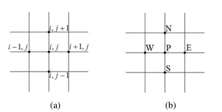
Figure 1:Five points in a uniform two-dimensional grid

where the subindices represent the location of the points in the grid.Thepoints P(central),W(west),E(east),N(north)and S(south)shown in Fig.1(b)correspond to the points(i,j),(i−1,j),(i+1,j),(i,j+1),(i,j−1)in Fig.1(a),respectively.

Considering hx=1/(Nx−1)and hy=1/(Ny−1),where Nxand Nydenote the number of points in the coordinate directions x and y, respectively, including the boundaries, we havethat:

for theinner points(P=2,···,N − 1)and aP=1,aW=aS=aN=aE=0,bP=SPin all boundaries.

3 Iterative methods and their orderings

Iterative methods are considered efficient in solving sparse and large systems [Burden, Faires and Burden (2016)].These methods are based on an initial guess for the solution, from which a sequence of approximations is built.Under certain conditions, the estimate converges to the exact solution of the system.In this work, the Gauss-Seidel method and some of its variants were used to solve the system of equations given by Eq.(5).

The Gauss-Seidel method can be classified as a pointwise solver and also as a multi-block solver (line by line, for instance).The difference between each solver is related to the way the unknowns are updated throughout the iterative process.

In point wise methods,each variable is updated individually.Fig.2 presents two classic orderings for the Gauss-Seidel pointwise method[Wienands and Joppich(2005)]:(a)Lexicographic ordering,and(b)Red-black ordering.Both orderings were used for comparison purposes.

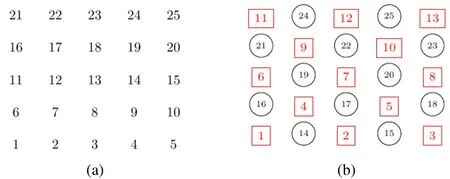
Figure 2:(a)Lexicographic;(b)Red-black orderings

In multi-block methods,each block is updated one at a time.Fig.3 shows two orderings for the Gauss-Seidel multi-block method:(a)x-line-GSand(b)y-line-GS.Fig.4 depicts(a)x-zebra-GSand(b)y-zebra-GS.

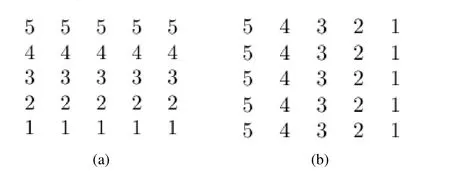
Figure3:Line ordering in the directions x(a)and y(b)

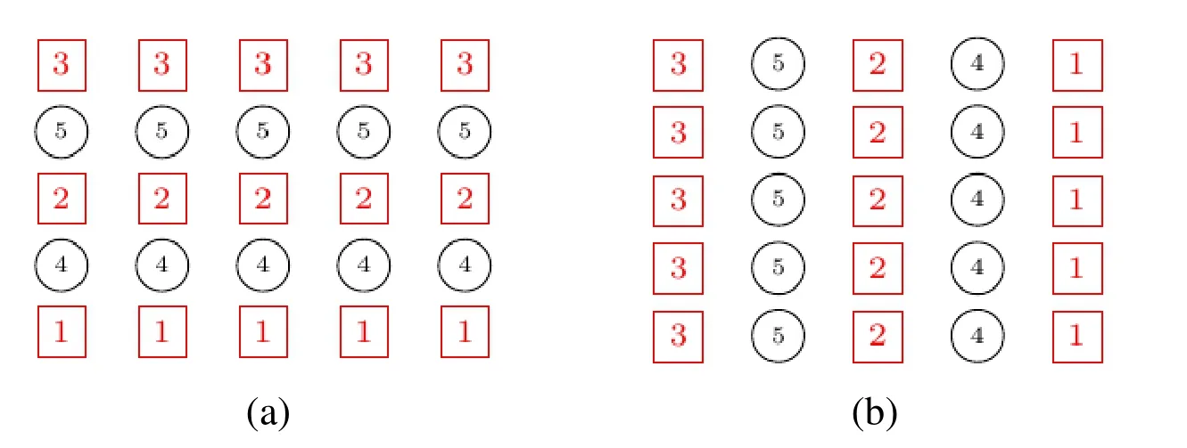
Figure4:Zebra ordering in the directions x(a)and y(b)

4 Multigrid method

In order to efficiently reduce the discretization error, very refined grids are used, thus generating large linear systems.Therefore, the multigrid is an alternative method to accelerate the convergence rate of the problems [Briggs, Henson and Mccormick (2000)].

The basic principles of the multigrid method are its smoothing and fine grid correctionproperties.Such technique involves transferring information of one problem through several grids, from the finest to the coarsest, so that all error frequencies are smoothed out.The transfer of information between grids is carried out by the restriction and prolongation operators.The way in which these grids are visited is called the multigrid cycle, such as theV-cycle shown in Fig.5.Several cycles can be executed successively until a stop criterion verified at the end of each cycle is achieved.

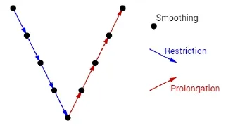
Figure 5:Diagram of a V-cycle applied to a problem with 5 grid levels

Eq.(1)was solved by the multigrid method,by employing CS scheme,V-cycle and zero initial guess.

Considering uniform grids,the grid coarsening ratio is defined as r=p/q,where q measures the spacing between the points of the fine grid(Ωh)and p measures the spacing between the points of the immediately coarser grid,denoted byΩH.In this study,r=2 was used(standard coarsening)[Wesseling and Oosterlee(2001)],thus H=2h.For study purposes,the linear system obtained from the discretization was solved by the different solvers(smoothers)with good smoothing properties described in Section 3.

5 Local Fourier Analysis(LFA)

LFA was carried out in order to determine the convergence factor for the two-grid algorithm[Trottenberg,Oosterlee and Schuller(2001)],which estimates the behavior of the asymptotic convergence of the multigrid.

The asymptotic convergence factorρ()=ρ2gis the spectral radius of the matrix,whereis the operator of two grids.Taking Shas the smoothing operator,ν1and ν2represent the number of pre-and post-smoothing iterations,respectively.The correction operator of the coarse grid is given bywhereare the prolongation and restriction transfer operators,respectively,L2h,Lhare the discrete Laplacian operators,and Ih,the identity operator in the fi ne grid.In this study,LFA was used to determine the asymptotic convergence factor of themultigrid,considering thesmoothers GS-LEX,GS-RB,x-line-GS,y-line-GS,x-zebra-GSand y-zebra-GS.

where,tκ∈ R are stencil coefficients(more details in Trottenberg et al.[Trottenberg,Oosterlee and Schuller (2001); Wienands and Joppich (2005)]).

where θ=(θ1,θ2) ∈ Flow=[π/2,π/2)2,in which Flowrepresents the low-frequency components,considering

These components are illustrated in Fig.6 [Trottenberg, Oosterlee and Schuller (2001)].The blank region represents the low frequencies, with components represented by (◦), and the hatched region represents the high frequencies, with the components represented by(·).

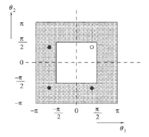
Figure6:Low and high frequencies[Trottenberg,Oosterleeand Schuller(2001)]

The operator Lhis represented by the matrix 4×4:

where,sκ∈ R are stencil coefficients(more details in Trottenberg et al.[Trottenberg,Oosterleeand Schuller(2001);Wienandsand Joppich(2005)]).

The discrete Laplace operators Lhand L2hare represented,respectively,by:

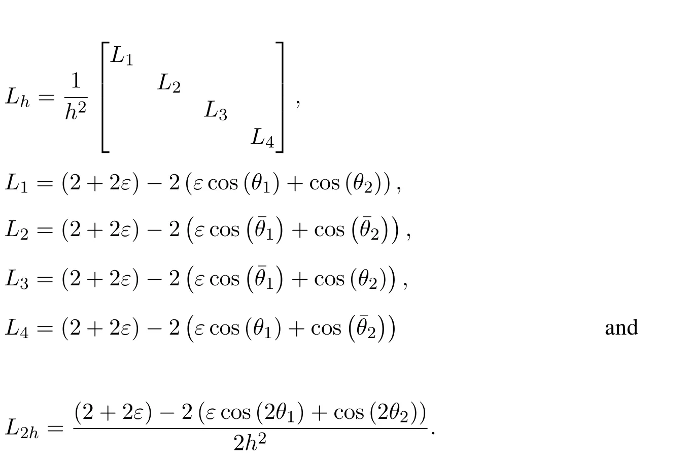
The smoothing operator Shisgiven by:

where

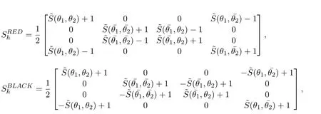
For the GS-RB smoother,the smoothing operatoris given by the product=

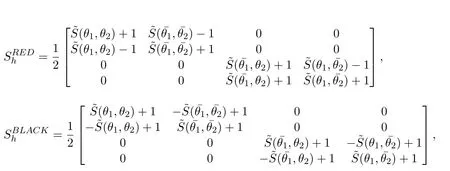
The GS-line smoother uses the operator given by Eq.(8),where(x,y)=(eiy)/(−2−2ε+εe-ix+e-iy+εeix)for thedirection x and˜S(x,y)=(eix)/(−2−2ε+εe-ix+e-iy+εeiy)for thedirection y[Wienands and Joppich(2005)].

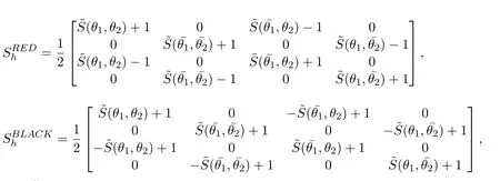
The x-zebra-GS smoother,similarly to GS-RB,isgiven by:

6 Numerical results

The results presented refer to the Eqs.(2), (3) and (4), with the domain = [0, 1]×[0, 1].It is expected that these results will be extended to larger domains.

In order to accelerate the convergence of the iterative methods, the geometric multigrid was used with zero initial guess,V-cycle and number of pre-and post-smoothing iterations ν1= ν2=1 and ν = ν1+ ν2.Since the problem investigated is linear,the multigrid was employed with the correction scheme,which is recommended for this case[Briggs,Henson and Mccormick(2000)].FW and bilinear interpolation were used as restriction and prolongation operators,respectively.

The infinity norm of the residual was used as stop criterion of the iterative process,nondimensionalized by the initial guess,that is,k Rnk∞/k Rnk0≤ tol,where Rnis the residual in the iteration n,R0is the residual in the initial guess and tol=10-9is the tolerance adopted.For every size of the problem N,the number of L levels employed was Lmax,in which Lmaxdenotes the highest possible number of levels that can be employed for a certain problem,considering N=3×3 points in the coarsest grid.For instance,if N=33×33 and r=2,the following group of grids is obtained:33×33,17×17,9×9,5×5,3×3,that is,Lmax=5.

The algorithms from this study concerning to the simulations were computed in Fortran 2003 language, using the Intel 9.1 Visual Fortran compiler with double precision.However, the algorithms concerning to the LFA were computed in MATLAB R2015a language.All simulations were performed in a computer with Intel Core i7 2.6 GHz processor, 8 GB RAM, 64-bit Windows 10, using double precision arithmetic.

The tCPUwas measured based on the CPU time function from Fortran,in which tCPUis defi ned as the time interval needed for generating the grids,establishing the initial guess,computing the coefficients and solving the linear system represented in Eq.(1)until the stop criterion established isachieved.

6.1 Preliminary results

In order to assess the level of reliability of the numerical solution, tests were performed toverify the codes that are part of the different smoothers studied.

Fig.7 presents the infinity norm of the numerical error versus N=5×5 up to 2049×2049 for all the smoothers studied,with anisotropy factor fixed atε=10-3.The results obtained show that,regardless of the smoother used,the errors were essentially the same(the biggest difference was of the order of 4.0×10-9)and decreased with the grid refinement.Fig.8 depicts the numerical error for the anisotropy coefficients assessed with N=5×5 up to 2049×2049,with fixed smoother(x-zebra-GS).Likewise,regardless of the coefficient of anisotropy,the errors were virtually the same(the biggest difference was of the order of 6.0×10-8)and decreased with the grid refinement.

According to Marchi et al.[Marchi and Silva (2002)], the apparent and effective orders of the numerical error are given, respectively, by:

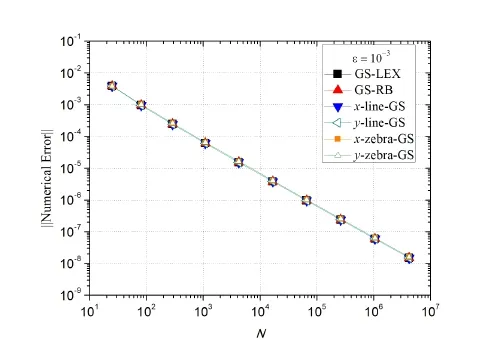
Figure 7:Infinite norm of the numerical error vs.N for the different smoothers, with anisotropy coefficient ε = 10-3

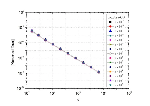
Figure 8:Numerical error vs.N for the x-zebra-GS smoother with several anisotropy coefficients

where φ1,φ2e φ3represent three solutions in three distinct grids with sizes h1,h2and h3,fine,coarse and super coarse grids,respectively,Φis the analytical solution and q=h2/h1=h3/h2isthe refi nement ratio.

Fig.9 shows that the apparent(pU)and effective(pE)orders for the infinity norm of the numerical error for the x-zebra-GS smoother tend to the asymptotic order,pL=2(due to the use of second order CDS)when the grid is refined.Tests carried out with different anisotropy coefficients and other smoothers demonstrated similar behavior to the onedepicted in Fig.9.

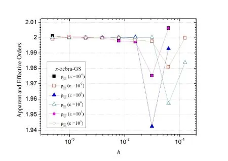
Figure 9:Apparent and effective orders vs.h for the infinity norm of the error, with x-zebra-GS smoother and the anisotropy coefficients ε = 1, 10-3 and 103

6.2 Asymptotic convergence factor

Fig.10 shows the convergence factor of two grids (ρ2g) calculated via LFA for each one of the smoothers assessed, for a problem N = 1025×1025.This data is presented for different anisotropy coefficients (ε).When the problem is isotropic (ε = 1), all solvers converge, 0 ＜ ρ2g≤ 0.2.It is possible to observe that for anisotropic problems, when ε ?1, only the y-line-GS and y-zebra-GS smoothers present good convergence factors, that is,ρ2g≈ 0, however, the GS-LEX, GS-RB, x-line-GS and x-zebra-GS smoothers diverge, that is, ρ2g≈ 1.On the other hand, for ε ? 1, x-line-GS and x-zebra-GS present better convergence factors than the other smoothers studied(GS-LEX,GS-RB,y-line-GS and y-zebra-GS),which confirms that block smoothers are more efficient than pointwise smoothers.Moreover,forε?1,there is strong coupling in the direction y(see Eq.(2)),therefore,line smoothers in this direction are more effi cient.Forε?1,there is strong coupling in the direction x,consequently,line smoothers in this direction are more effi cient.

Figure 10:Asymptotic convergence factor via LFA (ρ2g) vs.the anisotropy coefficient (ε)

According to Trottenberg et al.[Trottenberg, Oosterlee and Schuller (2001)], the computational cost (complexity) of the GS-line and GS-zebra smoothers is practically the same.However, one advantage of using the GS-zebra smoother is that its convergence factor for the multigrid is better than that of the GS-line smoother, as shown in Fig.10.

Considering the presented results and with the aim of developing a robust and efficient algorithm for solving the anisotropic problem in question (Eq.(2)), a variation of the zebra smoother called xy-zebra-GS is proposed.In this case, the x-zebra-GS is employed when ε? 1 and the y-zebra-GS is employed when ε ? 1, as shown by Algorithm 1.

For the proposed smoother, xy-zebra-GS, the asymptotic convergence factor of two grids(ρ2g), estimated by LFA, was compared with the empirical convergence factor (ρh),computed for a fine grid, obtained with ten levels of refinement (N = 1025×1025) and for different values of ε.Besides showing the robustness of Algorithm 1 in relation to different values of ε, Fig.11 highlights that the LFA provides extremely accurate predictions (of the order of 0.3×10-1) for the convergence factors, which confirms its importance as a preliminary analysis tool.

Algorithm 1:xy-zebra-GS

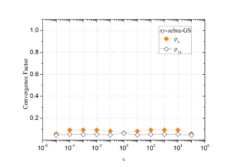
Figure 11:Asymptotic (ρ2g) and empirical (ρh) convergence factors for N = 1025×1025 v s.the anisotropy coefficient (ε)

The robustness of the proposed smoother, xy-zebra-GS, regarding the variation of N can be observed in Fig.12, in which the asymptotic convergence factor ρ2g, calculated via LFA, is compared with the ρhvalue, calculated empirically for different values of ε, in several grids (5×5 up to 2049×2049).Noticeably, for different values of ε and N, the convergence factor ph≈ 0.1 presents good results.

The smoother given by Algorithm 1 was used in all the following tests due to its efficiency and robustness.

6.3 Number of V-cycles

The number of V-cycles for each size of problem (5×5 up to 2049×2049) is shown in Table 1 for the xy-zebra-GS smoother proposed in this study.Only results for ε = 10a,a ∈ {0, 1, 2, 3, 4, 5, 6, 7} are presented, since results for ε = 10-aare quite similar.The number of V-cycles is roughly constant as the value of N increases, which is in agreement with the literature [Trottenberg, Oosterlee and Schuller (2001)].In addition, it is possible to notice that the proposed smoother needs few V-cycles regardless of the number of points N.

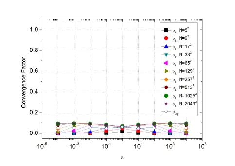
Figure 12:Asymptotic (ρ2g) and empirical (ρh) convergence factor obtained via LFA for grids N = 5×5 up to N = 2049×2049 versus the anisotropy coefficient (ε)

Table 1:V-cycles as function of the number of points N and different values of ε

6.4 Computational cost

In order to assess the computational cost of the xy-zebra-GS smoother,aprevious analysis of complexity based on theeffect of thenumber of unknownson the tCPUwascarried out.Consequently,several simulations were carried out considering isotropic and anisotropic problemswithε=10aandε=10-a,a∈{0,1,2,3,4,5,6,7}.

Fig.13 depictsa graph of the tCPUcurves for some anisotropy coefficients(ε)for several values of N.It was observed that the tCPUcurvesobtained forε=10-aare similar to the ones obtained forε=10a,in which a∈ {0,1,2,3,4,5,6,7},therefore,only the odd part of the latter are shown in thefigure.

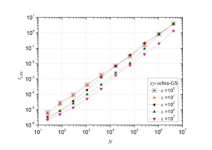
Figure 13:tCPU(s) vs.the number of points (N) for some values of ε

Finally, with the tCPUresults obtained using the xy-zebra-GS smoother, a geometrical adjustment of the type tCPU= cNpwas made in order to evaluate the performance of the multigrid, where c is a constant related to the method, p represents the order of complexity of the algorithm, or the gradient of the curve, and N is the size of the problem.Ideally, the multigrid method presents p = 1, which means that the tCPUincreases proportionally to the number of unknowns N [Wesseling (2004)].

The results of the geometrical adjustment are shown in Tab.2.Only the values of p and c for the anisotropy coeffi cients = 10a, a ∈ {0, 1, 2, 3, 4, 5, 6, 7} are d epicted.The results forε= 10-aare similar to the results for ε = 10a.These results confi rm that the tCPUof the multi grid with the xy-zebra-GS smoother grows roughly linearly with the increase of N, since in every case, p is near one.

7 Conclusion

The aim of this study was to propose an efficient and robust smoother for a two-dimensional diffusion problem with physical anisotropy.In order to reach the goal, it was necessary to perform a study of the convergence factor of the multi grid method for some smoothers by means of LFA.The geometrical multi grid method was employed with Correction Scheme,V-cycle, FW restriction, bilinear interpolation, zero initial guess and r = 2.The smoothers assessed were the well-known point wise smoothers GS-RB and GS-LEX, and the block smoothers x-line-GS, y-line-GS, x-zebra-GS and y-zebra-GS.The xy-zebra-GS smoother was proposed, which is a combination of the x-zebra-GS smoother with the y-zebra-GS smoother.The empirical and asymptotic convergence factor, the number of V-cycles and the computational cost according to the order of complexity of the smoother proposed were assessed.As result of this work, we verified that:

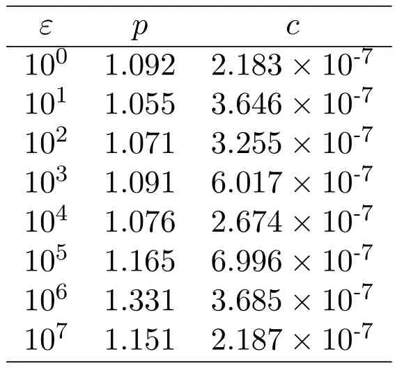
Table 2:Order of complexity p and the coefficient c regarding the coefficient of anisotropy ε

-The convergence factor computed empirically and by means of LFA resulted in very similar values, which confirms the importance and reliability of the LFA;

-Concerning to the smoothers assessed, the convergence factors of the block smoothers aremore efficient than those of the point smoothers;

-Among the block smoothers assessed, the zebra-GS presents the best convergence factors;

-Among all the smoothers assessed,the x-zebra-GS and y-zebra-GS have the best convergencefactor for 0＜ε?1 andε?1,respectively;

-In relation to the xy-zebra-GS smoother,proposed in this study,the number of V-cycles tends to beconstant as N increases;

-The xy-zebra-GS smoother presents good convergence factors and low computational cost regardless of the anisotropy factor,thus being a robust and efficient smoother for the anisotropic problem studied.

Acknowledgement:The authors would like to thank the Graduate Program in Numerical Methods in Engineering(PPGMNE)of the Federal University of Paraná(Brazil).This study was fi nancied partly by the Coordenação de Aperfeiçoamento de Pessoal de Nível Superior-Brasil(CAPES)-Finance Code001.