Kautz Function Based Continuous-Time Model Predictive Controller for Load Frequency Control in a Multi-Area Power System

A.Parassuram and P.Somasundaram

Abstract: A continuous-time Model Predictive Controller was proposed using Kautz function in order to improve the performance of Load Frequency Control (LFC).A dynamic model of an interconnected power system was used for Model Predictive Controller (MPC) design.MPC predicts the future trajectory of the dynamic model by calculating the optimal closed loop feedback gain matrix.In this paper, the optimal closed loop feedback gain matrix was calculated using Kautz function.Being an Orthonormal Basis Function (OBF), Kautz function has an advantage of solving complex pole-based nonlinear system.Genetic Algorithm (GA) was applied to optimally tune the Kautz function-based MPC.A constraint based on phase plane analysis was implemented with the cost function in order to improve the robustness of the Kautz function-based MPC.The proposed method was simulated with three area interconnected power system and the efficiency of the proposed method was measured and exhibited by comparing with conventional Proportional and Integral (PI) controller and Linear Quadratic Regulation (LQR).

Keywords: Load frequency control, model predictive controller, orthonormal basis function, kautz function, phase plane analysis, linear quadratic regulator, proportional and integral controller, genetic algorithm.

1 Introduction

In large electrical power systems, the load changes cannot be determined due to which the deviations occur in real and reactive power towards an unstable condition.So there is a need for continuous regulation of electric power generation for an efficient and reliable power system operation.The change in real power causes a change in frequency whereas the change in reactive power causes a change in voltage magnitude.Load Frequency Control (LFC) is a control strategy to minimize the tie line power and frequency deviations while at the same time maintaining the frequency within accepted limits[Saadat (1999); Kothari (2003)].

Utilizing fixed controllers is observed as conventional method to solve LFC problem.Fixed controllers such as Integral controller (I), Proportional-Integral (PI) and Proportional-Integral-Derivative (PID) controller are widely used in process control.However when the gain parameters are not properly selected, it often fails in achieving better output response [Mohamed, Bevrani, Hassan et al.(2011)].The electrical power system is nonlinear in nature [Zhu (2009)].So, the fixed controllers are not suitable for effective power system operation [Kumar and Suhag (2017)].

A number of investigations were conducted earlier suggesting various control techniques to solve LFC problem.A comparison of different controllers such as integral controller with the supervisor-selected weighting factors and the self-tuning regulator using recursive least square method for Load Frequency Control was performed in the literature[Agathoklis and Hamza (1984)].A brief summary of controlling strategies in LFC problem using traditional control methods, various energy sources, and control techniques based on adaptive and artificial intelligence in a deregulated power system were presented by Pappachen et al.[Pappachen and Fathima (2017)].

Model-based Predictive Control (MPC) is one of the process control techniques widely used in chemical industries, petroleum industries, automobiles and power systems.MPC uses a deterministic model of the system under consideration to predict future outputs and to obtain optimal control input signal by minimizing a cost function while at the same time, satisfying the system constraints as well.Since the deterministic model is used for optimization, it is ideal to overcome the LFC problem [Avci, Erkoc, Rahmani et al.(2013)].The MPC controller has the ability to manage multivariable constrained process in both supervisory level as well as in primary level control system [Wang (2009)].Further, it has the advantage of solving nonlinear problems [Minh and Rashid (2012)].

Recently, a number of researchers investigated the application of MPC to overcome LFC problem [Biyik and Husein (2018); Ersdal, Imsland, Uhlen et al.(2016); Zargar, Mufti and Lone (2017); Tang and McCalley (2016); Ma, Liu and Zhang (2017)].In the literature [Shiroei, Toulabi and Ranjbar (2013)], an MPC controller design was proposed considering the multivariable nature of LFC in MIMO, nonlinear problems such as Generation Rate Constraint (GRC) and various uncertainty problems in the system.MPC model based on grey theory for optimizing Battery Energy Storage System (BESS) in LFC problem was presented in Khalid et al.[Khalid and Savkin (2012)].An LFC problem for an interconnected power system of the Nordic power system was solved in one of the studies using MPC by considering power flow in tie-line power, maximum output power; generation limit, rate of change; in a generation, generator participation factors, tie-line power transfer margins through slack-variables and information on electricity pricing [Ersdal, Imsland and Uhlen (2016)].

Over the past few years, a number of attempts were made about the application of Orthonormal Basis Functions (OBF) in MPC control design.Some of the most commonly used OBFs are Laguerre and Kautz function.They are widely used in the field of applied mathematics, control theory, network synthesis, system identification and online parameterization [Kautz (1952)].Laguerre function seems to be suitable for well damped system with real poles, whereas Kautz function has an advantage of approximating system which is oscillatory in nature and it has complex poles [Oliveira,Amaral, Favier et al.(2000)].The purpose of LFC is to decrease oscillations in frequency deviations.So Kautz function is an apt solution for LFC problem.Only a limited number of studies were conducted regarding a combination of Kautz function with MPC algorithm.Kautz functions in MPC controller to improve control and stability of the autonomous car vehicle trajectory [Yakub and Mori (2014)].Discrete and continuoustime MPC with both Laguerre and Kautz function was designed and explained with simple examples in the literature [Wang (2009)].

This paper presents continuous-time MPC using Kautz function to solve LFC (Load Frequency Control) problem in an interconnected power system.A phase plane constraint was included in the optimization problem to ensure the stability of the system during uncertain disturbances.The proposed method was simulated in three area hydro-thermal interconnected power system.The results were compared with a conventional PI controller and LQR controller to prove the effectiveness of the proposed method.

2 Modeling of multi-area power system

The electrical power system was divided into a number of different areas.Each area was interconnected with its neighboring area through transmission lines called ‘tie lines’.In an interconnected power system, the load deviation leads to frequency deviation and tie line power deviation.LFC was used to maintain the frequency and tie line power within the desired limits in each area.Thus, in order for the LFC to be efficiently controlled, the design of dynamic LFC model was formulated considering both frequency as well as tie line power.In the current research work, thermal, hydro and wind power plant were considered for the study purpose.The basic block diagrams of thermal and hydropower plants in an interconnected system are shown in the Fig.1 and Fig.2 [Kumar (2017);Shiroei (2014)].The power system parameters considered for this study were listed in Appendix A.

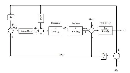
Figure 1:Block diagram of a Thermal power plant

The mathematical equations for the dynamic model of both thermal and hydro plants are as follows [Kumar and Suhag (2017); Shiroei and Ranjbar (2014); Bangal (2009)].Governor block (Thermal) is

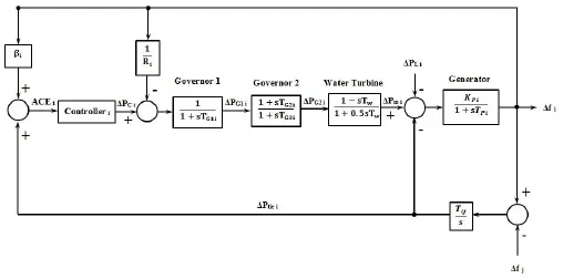
Figure 2:Block diagram of a Hydropower plant

Turbine block (Thermal) is

Stage 1 Governor Block (Hydro) is

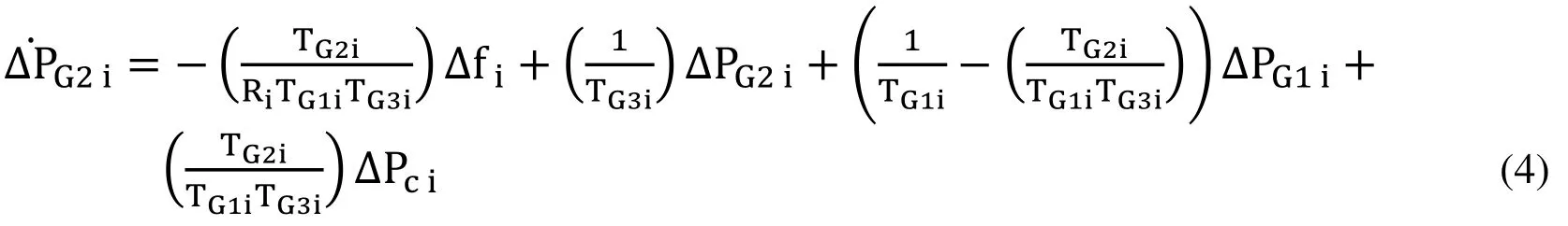
Stage 2 Governor Block (Hydro) is

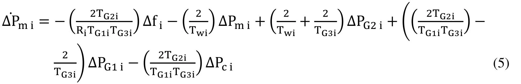
Turbine block (Hydro) is

The mathematical equations for frequency deviation and tie-line power flow are same for all the interconnected systems which are represented as follows:Frequency deviation is given by the equation

Tie line power flow is given by the equation

To maintain area frequency and tie-line power exchange with neighboring areas within the preset values, a supplementary control with a linear combination of frequency and the net interchange power for each area ‘i’ known as the Area Control Error (ACE) is to be reduced.

where

TGiThe speed governor time constant of the thermal power plant for area ‘i’

RiGain of speed droop feedback loop for area ‘i’

TTiThe turbine time constant of the thermal power plant for area ‘i’

KPiPower system gain for area ‘i’

TPiPower system time constant for area ‘i’

∆PgiThe incremental change in governor position of the thermal power plant for area ‘i’

∆PmiThe incremental change in turbine power for area ‘i’

TG1iThe stage 1 governor time constant of the hydropower plant for area ‘i’

TG2iThe stage 2 governor reset time of hydropower plant for area ‘i’

TG3iThe stage 2 governor time constant of the hydropower plant for area ‘i’

TwiThe turbine time constant of the hydropower plant for area ‘i’

∆PG1iThe incremental change in stage 1 governor position of the hydropower plant for area ‘i’

∆PG2iThe incremental change in stage 2 governor position of the hydropower plant for area ‘i’

∆PciThe incremental change in control input of area ‘i’

∆fiThe incremental change in frequency deviation for area ‘i’

TijThe synchronizing constant between area ‘i’ and area ‘j’

βiThe bias constant for area ‘i’

aijSynchronizing power coefficient

∆PtieiThe incremental change in tie-line power

∆PLiThe incremental change in load demand for area ‘i’

ACEiArea control error of area ‘i’

3 Approximation and realization

Some of the systems or network might be difficult to solve due to its nonlinear structure.Such systems need to be approximated for obtaining desired response [Kautz (1954);Magni and Scattolini (2004)].In approximation, the input function was approximated with some intermediate functions and then was optimized.Once the function was approximated to the desired form, it was converted back to a physically-realizable function.The basic steps of approximation are as follows:

Step 1:Simplification of function

In approximation theory, the first step is to express in detail about the operation or response of a function (which are difficult to analyze) in the form of simpler functions.If an arbitrary response f(t) is considered for a system which can be approximated by a Fourier series expansion over the interval (0, ∞) as

where φg(t) denotes a set of exponentially-damped sinusoids and orthogonal

CgThe coefficients of the expansion

Then the arbitrary response of the first ‘n’ terms is

Step 2:Determination of optimum pole locations

The location of the poles and zeros gives an approximate understanding of the system’s response characteristics.The roots of the characteristic equation, also known as eigenvalues of the system is equal to the poles of the system response.The proper selection of pole locations guides to the simplified form of the coefficient Cg.

Step 3:Orthonormal set

The orthonormal condition for the function φg(t),g=1,2,.over the interval (0, ∞)with unity weight is expressed as

Step 4:Formulation of Cg

The coefficient Cgis formulated and evaluated in terms of orthonormal set φg(t).

Step 5:Minimization of error

The mean-squared error between f(t) and f∗(t) has to be minimized to find the optimal pole location and to approximate the given arbitrary function identical to the physical system.If the f(t)is assumed as a piecewise continuous function, the integral squared error in an orthonormal expansion is given by the following equation

When expanding the Eq.(12) and assuming the error as ‘0’ then,

The Eq.(13) can be written as

Thus the equation (14) becomes the condition to be satisfied for proper convergence of the desired response.

4 Kautz function

The orthonormal basis functions are mostly used for system approximation and identification.A dynamic model with OBF gives approximate knowledge about the dominant dynamics such as time constants and damping factors of the system which can be included in the system identification process [Akcay and Ninness (1999)].Some of the orthonormal basis functions that are widely used are Laguerre base function and Kautz base function.Kautz functions are an extended generalization of Laguerre functions.Unlike Laguerre functions which only deal with identical real poles, Kautz functions possess the ability to approximate the system function with both real and complex poles.Thus Kautz function-based dynamic model can approximate the system in resonance.

4.1 Real pole

If all the poles are real, non-identical and all poles >0 whose pole locations lie at -p1, -p2… -pk…, -pN, then the Kautz network can be represented as

where k=2 … N and ‘N' is the maximum number of poles.

If all the pole locations are identical, then this is called a Laguerre function.

4.2 Complex pole

Let the non-identical complex poles are denoted as −αi± jβifor i=1,2,…,n where−αi＞ 0 for all i.Then Kautz networks with complex poles are represented as

4.3 State space form

Kautz functions can be expressed in a state space form as follows

where F(t),δ(t) and K(t) are the state vector, the unit impulse function and the Kautz network terms respectively.Ak, Bkand Ckare matrices determined by the locations of the poles.

5 Model predictive controller (MPC)

Model Predictive Controller (MPC) has the ability to solve multivariable problem and handle complex system constraints.These advantages make MPC a well suited option for power system and to overcome LFC problem [Shiroei, Toulabi and Ranjbar (2013)].MPC uses the explicit model to predict the future response of the system.It calculates the controller input by solving objective function with constraints through optimization.Once the optimal trajectory of the future response of the system was calculated, only the first input sample of the control signal would be taken for system processes based on Receding Horizon Control (RHC) whereas the remaining input samples are ignored.This optimization is performed again for next time instant with a new set of system information.

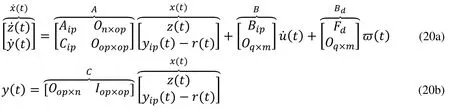
State space model is the most common type of MPC structure used to represent the dynamical system.The mathematical model of a linear time-invariant multivariable system with ip-input,op-output,d-disturbances and n-states can be expressed in a state space form as follows:

where xip(t),yip(t),u(t) and w(t)are state vector, output vector, control vector, and disturbance vector respectively.The matrix coefficients Aip,Bip, Fdand Cipare system matrix, the input matrix and disturbance matrix respectively.The number of output op should be less than the number of input ip.

6 Kautz function-based MPC (K-MPC)

The modeling and implementation of the Kautz function-based MPC controller for continuous-time application are described here as per the literature [Wang (2009)].The K-MPC method was designed by describing system model in continuous-time while computations of the optimization problem were performed in discrete time (in off-line)[Minh and Rashid (2012); Magni and Scattolini (2004)].The optimization problem for control trajectory included manipulated variables whereas its optimal tuning using GA is explained below.

6.1 Modeling trajectory of the future control signal

The moving time window of the optimization process is assumed to be between ti≤t≤ti+Tp.‘ ti’ is considered as the current time and ‘Tp’ as the maximum duration of the moving time window.The Eq.(14) stated that, for a stable closed loop system, the control trajectory u(t) should converge exponentially to zero when there is a transient state response due to load disturbance.If the disturbance is continuous, then the control trajectory u(t) converges to a specific constant value, instead of zero.So, it is wise to optimize derivative of the control trajectory u̇(t).The derivative of the control trajectory u̇(t) is expressed as follows

6.2 Augmented state space model

As the Eq.(19) concludes, there is a need for integral action occurs once the derivative of the control trajectory was obtained.So the design of system state space model need to be modified to an augmented state space form.With an assumption that z(t)=̇ is the augmented state space form of (18a) and (18b) with u̇(t) as control input, this can be defined as follows.

Where I an identity matrix

O A zero matrix

u̇(t)A derivative of the control trajectory

ϖ(t)Continuous-time integrated zero-mean white noise

r(t)A constant vector of a reference signal

The dimension of the augmented state space is n2=n+op.

6.3 Selection of poles

Kautz function requires the optimal selection of poles.The poles can be calculated from the priori information of Linear Quadratic Regulator (LQR) using the augmented state space model of the system to be solved.The closed-loop eigenvalues of the system are calculated by solving the characteristic equation

where A and B are matrix coefficients of an augmented state space model, λ is the eigenvalues of system matrix(A−BKlqr), I is an identity matrix and Klqris a gain matrix obtained by minimizing the cost function of LQR over a finite time horizon.Assuming Q=CTC, the quadratic cost function of the LQR is expressed as:

where Rlqr=rlqrIip×ip, C is a matrix coefficient of augmented state space model of the system, rlqris a constant multiplier and Iip×ipis an identity matrix.

6.4 Computation of Kautz function

The optimal poles (eigenvalues), obtained by solving the Eq.(21), was used for the computation of Kautz network.Then this Kautz network terms again were used for calculating the state space parameters of (17a) and (17b).Kautz function, using state space parameters, is defined as

where i=1,2,…,ip

When substituting (23) in (19), it gives the derivative of the control trajectory u̇(t) in terms of Kautz function as

where K(t)is a Kautz function andis the vector of coefficients.

6.5 Design of optimal controller

The main objective of the K-MPC is to design an optimal control trajectory for MPC by minimizing the quadratic cost function.The optimal control trajectory u̇(τ) is designed using a controller gain matrix Kmpc.Assuming that there is a time ‘τ’ which lies within the interval 0≤τ≤Tpand Q=CTC, the optimal cost function of a system is expressed as:

where

As the first term of (25) is negligible and it is the only term in the cost function dependent on, the optimalis

6.6 Computation of Coefficient vector

The cost function Eq.(25) clearly states that the coefficient vectorplays a vital role in the design of the control trajectory.The vector of coefficientsis calculated from the Eq.(28).The computation ofrequires Ω and Ψ.

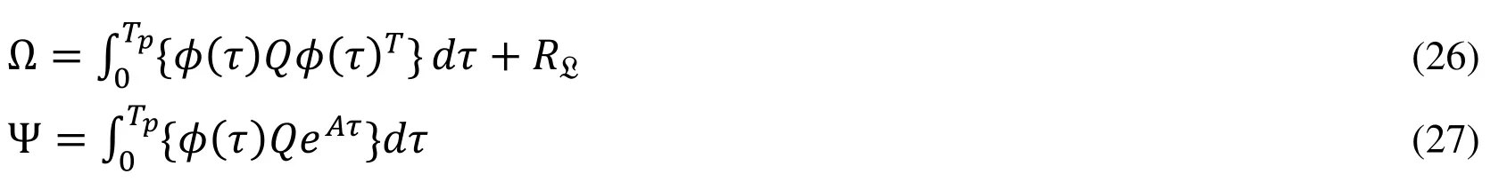
6.6.1 Computation of matrices Ω and Ψ

The matrices Ω and Ψcan be evaluated using the Eqs.(26) and (27) in discrete form as they do not rely on current time ti.By dividing time τ in discrete as τ=0,ℏ,…,Mℏ,such that Tp=Mℏ, the matrices Ω and Ψcan be evaluated as follows:

The matrices Ω and Ψ are the functions of φ(τ).So φ(τ) has to be calculated first followed by φ(τ) can be calculated by computing(τ)T.The i-th input of the convolution integral(τ)Tis obtained by solving the linear algebraic equation

Above equation is solved in discrete form to obtain optimalAfteis calculated, φi(τ)Tcan be calculated by substitutingin

6.6.3 Implementation of control signal

According to Receding Horizon Control (RHC), the first signal of u̇(t) alone is considered for the control input of the system.Assuming a random time ‘t’, the derivative of the optimal control is

where

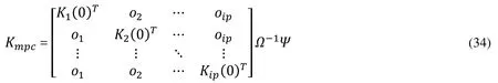
u̇(t)can be again defined by splitting Kmpcinto state and output component as,

where Kxand Kyare the gain matrices for state variables and system output.

Kyis a diagonal matrix with each diagonal values, a gain value of the integral controller.Finally, the control trajectory was obtained by integrating the derivative of the control trajectory.Therefore,

Substituting the Eq.(35) in (36), the control trajectory in terms of state variables is given by

where r(t) is a reference signal.

7 Evaluation of system response

To evaluate the response of a closed loop system, the root of the characteristic equation of the closed-loop system is required.To find the response of the system, the derivative of the control trajectory (33) is substituted in (20 a).Then, (20a) and (20b),

Solving (38 a) and (38 b) using Laplace transformation,

The Eq.(39) is the system output response of the closed loop feedback system in ‘s’domain.By taking the inverse Laplace transform of the Eq.(39) results in the differential equation of the system is obtained in time domain.This differential equation is used as the input for the objective function for optimization in the following section.

8 Constrained optimization problem

In this paper, to obtain an optimal controlled response, one of the well-known performance criteria was used as an objective function.An Integral Absolute Error (IAE)is a performance measure which integrates absolute of error over time.Let Jminbe the objective function to be solved.The objective function is given by

Subject to,

where

D = Determinant of (A−BKmpc)

λ = Eigenvalues of (A−BKmpc)

To ensure the stability of the system, the Eq.(41) was implemented into the system cost function as a penalty factor.Stability constraints were applied as a penalty factor in the cost function of MPC problem [Magni and Scattolini (2004)].Inserting stability constraints in optimization problem for uncertainty is described in the literature as well[Bemporad and Morari (1999)].

9 Phase-plane analysis of eigenvalues

In this paper, a new technique was proposed by implementing the constraints using penalty factor in the cost function, by phase plane analysis, in order to determine an optimal solution in MPC such that the system remains stable.

Phase plane analysis is an analysis method to observe the features of a dynamic system in a graphical manner.To observe the system behavior, the solution of the system at equilibrium is to be determined which is called a ‘critical point’ and the vector plane that represents the behavior of the system is known as ‘phase portrait’.The path of the solution in phase portrait is viewed as a moving particle in a curve or line.Eigenvalues and eigenvectors are the most convenient ways of representing the differential equation for phase plane analysis.Depending on whether the eigenvalues are real or complex and positive or negative, the system behavior can be determined as stable or not.This kind of analysis is well suitable for oscillatory systems.

10 Optimal tuning of Kmpc

The eigenvalues of the system matrix (A−BKmpc) are the poles of the given system.The gain matrix Kmpchas to be selected optimally for a stable operation of the system.The optimal Kmpcensures the derivative of the control trajectory to exponentially decay to zero.For optimal Kmpc, the parameters such as rlqr, ℏ, Tp, RKand Kyhave to be fine tuned.

There are several optimization algorithms available for finding optimal solution for the given optimization problem.If the optimization problem is a multimodal type, then conventional iterative type algorithm cannot guarantee an optimal solution.As the multiarea power system is a complex and nonlinear problem, which is difficult to optimize with conventional methods, a meta-heuristic algorithm such as the Genetic Algorithm was applied to the proposed methodology for optimal tuning.

10.1 Genetic algorithm

Genetic Algorithm (GA) is an Evolutionary Algorithm (EA) based on Charles Darwin theory of natural evolutionary process in biological systems.GA is a prominent optimization algorithm which can hold large search space and has a greater chance of determining the global best solution for an optimization problem [McCall (2005)].GA also has the capability to handle multiple variables which makes it suitable for solving both constraint and unconstraint optimization problems.

The standard procedure of GA consists of biologically-inspired operators known as selection, crossover, and mutation [Rao, Rao and Dattaguru (2004)].GA starts with the initialization of the population and the population consists of individuals whom are randomly generated.Each individual of the population is represented as ‘real value’ or‘strings’.At each generation, the potential of every chromosome is evaluated with a value known as ‘fitness’ by solving the objective function.Once the fitness of each chromosome is evaluated, GA chooses healthier chromosomes among all the chromosomes based on fitness value.Crossover is a recombination of chromosomes from the selection process to form a new set of chromosomes.In mutation process, every gene position, in an individual chromosome of a newly-produced chromosome, is interchanged with randomly generated numbers to form a new population for next generation.The whole process is repeated again with the new population produced after mutation until the best solution is reached or a stopping criterion is reached.

10.2 Algorithm steps for the proposed methodology

The proposed methodology to tune Kmpcwith GA algorithm is summarized in the following steps:

Step 1 Initialize GA parameters such as search space S, number of chromosomes ℂ,number of generations G, crossover rate Cℛ and mutation rate ℳℛ.

Step 2 Initialize populations ℙ for search parameters rlqr, ℏ, Tp, RKand Kywith random values and set generation counter as 0.

Step 3 Calculate eigenvalues using LQR with parameter rlqr.

Step 4 Calculate Kautz state space matrices Ak,Bkand Ckwith eigenvalues.

Step 5 Calculate Kautz function K(t).

Step 6 Calculate convolution integral φ(τ).

Step 7 Calculate matrices Ω and Ψ with parameters ℏ, Tpand RK.

Step 8 Calculate the feedback gain matrix Kmpcwith parameter Ky.

Step 9 Evaluate the system response using (A−BKmpc).

Step 10 Evaluate the fitness value for each chromosome in the current generation.

Step 11 For each population, the parent chromosomes are selected based on fitness values.

Step 12 Parent chromosomes are assigned with random numbers ‘rp’.If Cℛ ＞ rp,crossover takes place and new children are produced.Else no children are produced.

Step 13 The child chromosomes are assigned with random numbers ‘cp’.If ℳℛ ＞ cp,mutation takes place and the new population is produced.

Step 14 Increment the counter and repeat the steps 3 to 12 till the stopping criterion is reached.

Step 15 The final solution is the parameters to form optimal Kmpc.

11 Simulation results and discussion

The three area power system examples from the literature [Bangal (2009)] were used for the simulation.Area 1 and Area 2 were two identical thermal non-reheat power plants whereas Area 3 was a hydropower plant.The dynamic system for MPC was designed assuming that all the areas would be provided with load change.The experiment was conducted using two case studies.In Case 1, a step load was applied to area 1 and area 2 alone whereas in the Case 2, step load change was applied to all areas.In both the cases, step load change with magnitude 0.1 pu was applied at a time instant of 10 s.The system responses were compared with conventional PI controller, LQR and Kautz function-based MPC (K-MPC).

Case 1:The output responses for the case study 1 are shown in the Fig.3.In case 1, all three controller performances were found to be almost identical.As area 3 was not applied with step load change, the oscillations in both frequency deviation and tie line power of area 3 alone were much lesser when compared to other two area frequency deviation and tie line power.Oscillations in area 2 responses were more.All controller outputs were stable even if the system was modeled assuming all areas would have the same load.But none of the controller performances seem to be optimal for all the three areas.Area 1 system output for LQR was better than both K-MPC and PI.Area 2 system output for K-MPC was better than both LQR and PI.PI controller showed much lesser performance than both K-MPC and LQR.

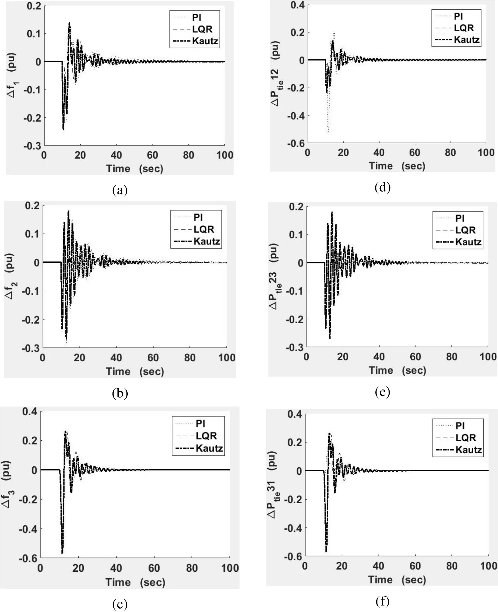
Figure 3:Output responses of case study 1

Case 2:In this case, all the areas were provided with step load change.The output responses for case study 2 are shown in the Fig.4.It is evident from the comparison of output responses that the proposed method exhibited optimal performance when compared to other two controllers.The responses of the PI controller were better than LQR unlike as in Case 1.LQR struggled to maintain the stability of system response.

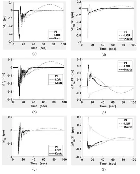
Figure 4:Output responses of case study 2

12 Conclusion

A Kautz function-based MPC (K-MPC) with phase plane stability was proposed for the optimal control of LFC problem.For simplicity, the design of the MPC used in this problem is of a centralized type.GA was presented to optimize the parameters of K-MPC.To prove the efficiency and robustness of the proposed method, it was examined on a multi-area interconnected power system problem that consisted of two thermal non-reheat power plants and a hydropower plant through simulation.Simulations were carried out using MATLABSimulink.The experiment was conducted as two case studies by including and excluding the load in the hydropower plant.The K-MPC is basically a PI controller.So, the proposed method was compared with both LQR and the conventional PI controller.The simulation results inferred that when the stability constraint is included in the cost function, the proposed method is able to provide reliable and stable closed loop output, even in case of any uncertainties present in the system.If the proposed method is implemented in the system without uncertainties, it is predicted to have better performance than other methods.

Acknowledgment:The author would like to thank all faculties of Anna University,Chennai for their guidance and valuable suggestions for the completion of this project.

Appendix A.System data

Area 1Area 2Area 3Tie-lineB1=0.425 pu.MW/Hz R1=2.4 Hz/pu.MW Tg1=0.08 s Tt1=0.4 s Kp1=120 Hz/pu.MW Tp1=20 s B2=0.425 pu.MW/Hz R2=2.4 Hz/pu.MW Tg2=0.08 s Tt2=0.4 s Kp2=120 Hz/pu.MW Tp2=20 s B3=0.425 pu.MW/Hz R3=2.4 Hz/pu.MW T1=48.7 s T2=0.5114 s T3=10 s Tw=1 s Kp3=120 Hz/pu.MW Tp3=20 s T12=0.4442 pu.MW T13=0.4442 pu.MW T23=0.4442 pu.MW a12=-1 a13=-1 a23=-1