Blood Flow Simulation in the Femoral Artery

Camilo A. Naranjo | Andrés F. Villa | Juan C. Vélez | Ricardo A. Prato | Alberto J.Cadena | Juan P. Tello*

Abstract—This paper presents the development of the blood flow simulation in two dimensions over the real geometry of the femoral artery. The Navier-Stokes equations are solved using the finite element method, to obtain the distributions of the blood pressure and flow velocity in multiple instants of time and different places of the femoral artery and thus determine the current condition of the blood vessels. The velocity field shows a laminar behavior,where, the velocity is higher in the center of the artery and decreases as the blood flow approaches artery walls. In spite of all artery and blood flow properties not being considered, the values of pressure and velocity obtained are within the normal ranges. Finally the model is used to verify if there exist irregularities in the blood flow in both healthy subjects and sick patients.

1. Introduction

The human circulatory system is a closed system in which blood flows through the arteries with high pressure and comes back through the veins with low pressure. The ascending aorta artery has an elastic behavior that helps maintain a continuous flow despite the pulsatile pumping of the heart; this phenomenon is known as the Windkessel effect[1]. As human gets older, the arteries lose elasticity and the ability to absorb pressure, causing increased blood pressure and stress in the wall of arteries leading to disease known as arteriosclerosis.

Arteriosclerosis is an abnormal proliferation of tissue in vessels where they are not usually found, invading them and altering their hemodynamic. These alterations produce a progressive decrease of blood flow towards organs and tissues. Once the obstruction reaches a critical threshold, the blood flow is reduced significantly and ischemia occurs in the affected region. Ischemia is a consequence of decreased blood flow, causing nutrient input to tissues to be insufficient for metabolic activities. Ischemia can cause the death of the affected tissues, making limb amputation necessary[1],[2]. Numerical simulations have been used for better understanding and prediction of conditions triggering diseases such as aortic aneurysm and arteriosclerosis[3].

Other pathologies with hematological origin like leukemia, hemolytic anemia, and thalassemia or pathologies associated with the risk factors of thrombosis and atherosclerosis like myocardial infarction, hypertension, strokes,or diabetes are mainly related to the disturbances of local homeostasis[4].

In [5], Simoncinni et al. developed a procedure to segment patient’s hepatic arterial vasculature with a Hessian based approach on three-dimensional angiography, and to perform blood flow numerical simulation in the extracted geometry with ANSYS Fluent. In vivo blood velocity measurements were performed using phase contrast magnetic resonance imaging to constrain these simulations.

This work starts by analyzing a mathematical model, which can determine the alterations of blood flow in the femoral artery of a patient. The model is based on the Navier-Stokes equations, which governs fluid behavior and allows for the calculation of pressure and velocity fields[6]. The finite element method (FEM) is used to approximate the solution of the model. The geometry of the femoral artery is obtained through an angiography, using a computer axial tomography (CAT) scanner[6]. Once the images are acquired, they are processed and a threedimensional reconstruction of the artery is performed. Subsequently, a view of 10 cm (two-dimensional plane) is selected, bearing in mind that the section must contain most of the alterations of the artery to observe changes in pressure and velocity of blood flow.

Some considerations are taken into account to develop the modeling and simulation, such as, artery’s walls stiff and incompressible blood flow with constant density and viscosity[6]-[11]. Also, in most parts of the arterial system, blood flow is Newtonian in normal physiological conditions[3],[4].

There are different works in blood flow simulation, some use commercial software such as ANSYS, FEA,CDF, COMSOL and others of free access and distribution and some own of investigation centers such as, the GID software of the International Center of numerical methods in Engineering—CIMNE. For example, the Colorado Health Science Center analyses a case study by using a mechanisc-based model of varying complexity to gain insight into pulmonary arterial hypertension (PAH) for the development of new disease diagnostic using the ANSYS commercial software[12]. In [13], Oshima et al. developed a numerical simulation system for the study of a cerebral aneurysm. In this study they used the commercial visualization software AVS to obtain the three-dimensional structure, and then, transferred it to the automatic mesh generation software, ICEM CFD to create the finite element mesh. The simulation results are visualized by using the commercial visualization software FIELD VIEW. The characteristic of the software developed is the possibility of modifying each one of the lines of code, such that the algorithm used to solve the problem should be adapted to the different physical structures that can be obtained from the morphological diversity data that patient could have in particular.

The aim of this work is to create a simple and low cost model, to calculate the blood pressure and flow velocity in multiple instants of time and different places of the femoral artery, as part of an early diagnosis. This process allows to determine the irregularities in the blood flow in both healthy subjects and sick patients, and also the current condition of the blood vessels.

The model of blood flow in the femoral artery begins with the solution of an FEM applied to a two-dimensional image obtained from the three-dimensional reconstruction of the artery. Later, a Matlab-based software tool for flow simulation is proposed. Finally, the distributions of the blood pressure and flow velocity are displayed in a graphical user interface.

2. Methodology

The tool developed is divided into four stages (see Fig. 1). In the first stage, the mathematical model based on Navier-Stokes equations is implemented using the FEM to approximate the geometry of the artery. In the second stage, the CAT images are taken and a three-dimensional reconstruction of the section to be processed is performed. From the reconstructed model a two-dimensional section of 10 cm is chosen. The third stage consists of the simulation of the blood flow in the selected area to finally visualize the model through a graphical user interface (GUI) developed for this purpose.

Fig. 1. Block diagram of the project.

2.1. Implementation of the Mathematical Model

The FEM is used to solve numerically the Navier-Stokes equations[14]. We considerbe a shape-regular,quasi-uniform triangulation into triangles with mesh sizeon the domain, making use of Taylor-Hood elements that guarantee the stability of the numerical solution and therefore a good convergence[15].

The Taylor-Hood elements use quadratic functions and linear functions, for all,to approximate the pressureand velocityrespectively.

Considering that the Navier-Stokes equations have a non-linearity and a time-dependent term, we precede to divide the problem into three stages (see Fig. 2)[7],[15].

Fig. 2. Stage of the development of mathematical model.

1) Linear analysis: This stage corresponds to the analysis of the Stokes equations which are obtained by studying the linearization of the static case of the Navier-Stokes equations. That is, removing the second summand of the first term from (1) we obtain

The solution of this case is done by mixed finite element method (MFEM), which allows solving two variables simultaneously. Letbe a basis of quadratic functions andbe a basis of linear functions on, then the approximate functions ofandhave, respectively, the formsWithout lo ss of generality, for convenience, we setandetup, the analysis beings with the reduction of the problem posed as in (1) can be changed to an equivalent matrix problem of the form[15]as

2) Nonlinear analysis: It is obtained by discarding the time derivative and proceeding to solve the nonlinearity using the Newton-Raphson method. The linearization process produces additional terms that lead to the matrix system for each Newton iteration taking the form described as[15]

3) Temporal analysis: The system of equations discussed only depends on space, while that in (1) depends on space and time. At this stage the calculations are performed using the backward Euler method[7],[16]. This is why the matrix system of (4) is modified with the time-dependent term M/Δt[16], as in (5).

where M/Δt is the ratio between the mass matrix and the selected time step.

Taking into account that the blood flow is the variable to be simulated, a time stepis defined according to the duration of the cardiac cycle, which has an average duration of 0.8 s. That is,and[10],[11]. A number of steps that allow for an appropriate resolution from a computational and medical point of view are selected. 60 is a consistent value considered for the study, resulting in a step time of 0.0133 s, as in (6).

2.2. Reconstruction of the Artery

An angiogram is performed on an anonymous 21-year-old patient. The digital imaging and communications in medicine (DICOM) images obtained (see Fig. 3) are processed, using a rendering algorithm previously developed,a three-dimensional model of the femoral artery of the left leg is created. The next step is to transform the threedimensional model into a two-dimensional image, taking a view and then a section of 10 cm in length as shown in Fig. 4.

Fig. 3. CAT images of patient’s lower limbs.

The image of Fig. 4 is processed in two stages. In the first stage, the noise and sections of the artery that are not the parts of the femoral artery are reduced; furthermore, a straight cut is made at the ends, generating the image shown in Fig. 5.

Fig. 4. Geometry in two dimensions obtained from the reconstruction.

Fig. 5. Geometry in two dimensions obtained after the first step.

The straight cut is made to ensure that the flow direction is always normal to the surface of the ends.This consideration allows simplifying the calculation of the boundary conditions, that is why the directional derivate of velocity becomes equal to zero[8],[17]. In the second stage, the image is subjected to a media filter and then smoothed using a polynomial interpolation algorithm of order 10. In addition, a scale transformation (pixels to meters) is performed because the dimensions of the image are widened. The geometry of the artery after being processed is shown in Fig. 6.

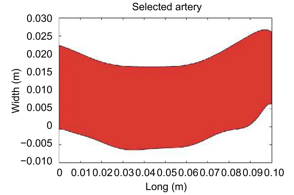
Fig. 6. Geometry in two dimensions obtained after the second step.

2.3. Simulation of Blood Flow on the Reconstructed Artery

The simulation stage consists of the combined results from the first and second stages. In order to develop the simulation correctly, it is necessary to specify the boundary conditions of the blood flow on each one of the arterial walls[15]. The boundary conditions for the selected artery were obtained by some data present in the bibliography[8]-[11].

Although the boundary conditions were not calculated directly, the data taken from the literature allowed getting a very realistic model. Also, the artery was considered as a rigid tube, with neither elastic nor flexible walls.Consequently, in the simulation, the interaction between the blood and the arterial wall was disregarded. The blood behaves as a second order fluid, that is, a non-Newtonian fluid. This means that viscosity depends on velocity gradient, temperature, and pressure[1],[7]. Thus, to avoid a high complex mathematical model, blood was considered as a first order or Newtonian fluid with constant viscosity and incomprehensible[7].

Fig. 7. Domain of the element and distribution of boundary conditions.

The simulation values used were viscosityand density

[8]-[11]. Furthermore,three boundary conditions were defined: One for the superior and inferior walls, corresponding to the Dirichlet boundary conditions. The second condition located on the inlet artery, also matching the Dirichlet boundary conditions. To conclude, a final boundary condition locates on the outlet artery, correlating with the Neumann boundary conditions[7],[15]. Fig. 7 shows the domain of each element and the boundary conditions distribution[15],[17].

▪ Boundary conditions on top and bottom artery walls: The boundary conditions on the arterial walls are attached to velocities equal to zero[8]-[11].

▪ Boundary conditions on the inlet of the artery: It consists of a velocity profilewhere each velocity value was measured in the femoral artery with an invasive method. The maximum velocity is 34.7 cm/s[11]. This boundary condition takes the shape of a sinusoidal function with an amplitude of 34.7 cm/s, as in (7).

where f is the cardiac frequency equal to 1.25 Hz and t is the time, which ranges between 0 and 0.8 s.

▪ Boundary conditions for the outlet of the artery: The boundary condition on the outlet of the artery is attached to a zero pressure value[8]-[11].

The velocity and pressure meshes generated to carry out the simulation are shown in Fig. 8.

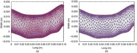
Fig. 8. Meshes to carry out the simulation: (a) velocity and (b) pressure.

2.4. Design of the Graphic User Interface

The simulation of the blood flow is visualized on a GUI made in Matlab. This tool allows selecting the figure of the geometry of the artery, putting the artery dimensions, specifying the temporal resolution, and selecting the number of steps to be simulated. Fig. 9 shows the execution of the simulation and the visualization tool.

3. Results

This paper focuses on the development of a simulation tool for blood flow, pressure, and velocity analysis in the femoral artery. A 21-year-old patient was selected as a candidate for an angiography with computed tomography(CT) at Clínica de la Costa in Barranquilla. As a result, 150 images were obtained, from which an arterial threedimensional model was reconstructed. Then, a two-dimensional view of the artery was built to look for geometry irregularities and detect visible changes in blood flow performance.

Despite the simulation of the real artery, it was necessary to use some values extracted from the literature to supply the mathematical model solution for complex fluid behaviors (Navier-Stokes equations). However, the same considerations are kept in mind by other authors that have worked with related issues. The blood flow computational simulation tool developed in this project shows the pressure and velocity in a graphic user interface.

Fig. 9. Block diagram of the simulation tool.

Fig. 10 shows the performance of the velocity of x-axe and y-axe components for two time intervals. It should be noted in the laminar fluid behavior, how the minimum velocity is near the artery walls and the maximum is reached at the artery longitudinal middle axe.

This behavior agrees with the theory and the considerations taken for the simulation. The resultant velocity values do not exceed the maximum velocity threshold presented in the scientific bibliography, vmax=34.7 cm/s[11].

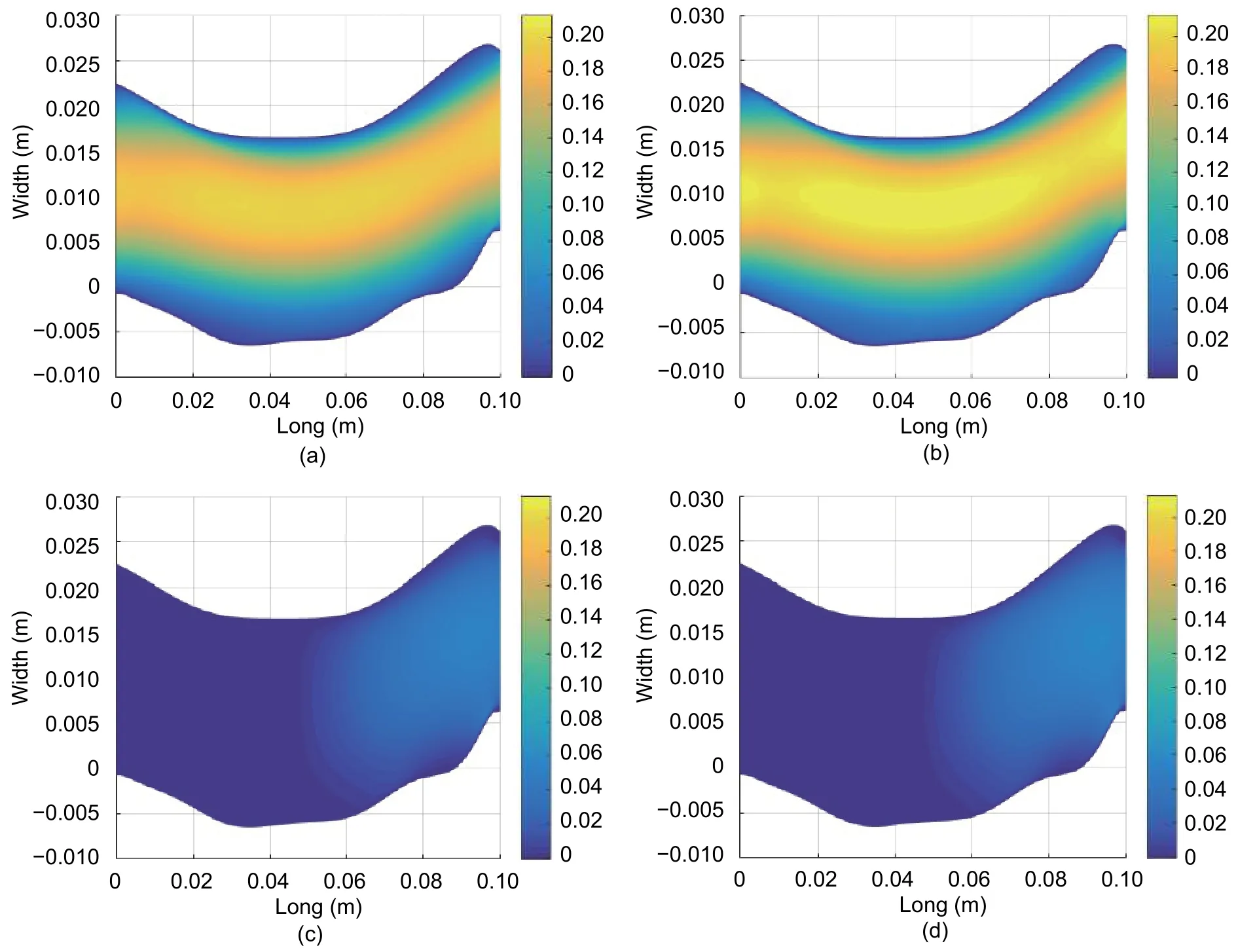
Fig. 10. Simulated results of the blood flow: x-velocity (m/s) for (a) t=0.0133 s and (b) t=0.0267 s; y-velocity (m/s) for (c)t=0.0133 s and (d) t=0.0267 s.

On the other hand, the velocity’s y-axe component presents very short values compared with the ones from the x-axe component, showing the tendency of the blood towards a laminar behavior. Due to this laminar profile,the y-axe velocity increases when closer to the artery outlet. The artery curve at the outlet may be a reason for y-velocity to increase in order to maintain this denoted laminar behavior.

Fig. 11 shows the blood flow velocity magnitude and direction. Velocity direction (arrows) follows the curve of the artery and, maintains the laminar profile, considered at the start of the simulation.

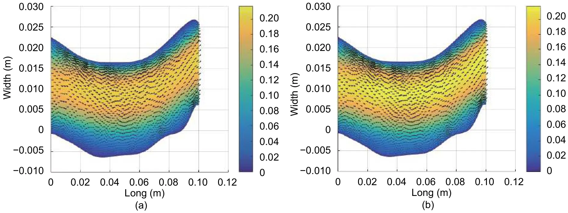
Fig. 11. Magnitude and direction of the velocity (m/s): (a) t=0.0133 s and (b) t=0.0267 s.

Fig. 12 shows the results for blood pressure. The values fall within a normal pressure range (80 mmHg to 120 mmHg)[1],[9],[11]. However, at the outlet of the femoral artery, pressure remains less than 80 mmHg. This value is the result of a boundary condition that is attached with pressure equal to zero in this region. Moreover, the region of study was assumed as an isolated region and did not consider the real interactions of the other circulatory systems.This is the reference for measuring the pressure in other points of the artery.

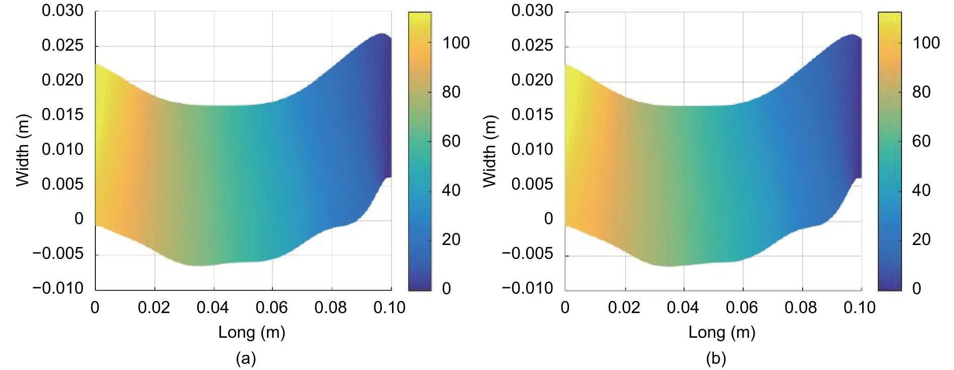
Fig. 12. Simulated results of the blood flow pressure (mmHg) in (a) t=0.0133 s and (b) t=0.0267 s.

4. Discussion

For the development of the tool, a mathematical model that solves the Navier-Stokes equations through the FEM, was implemented. This model presents the expected trend in which the error decreases with an increasing number of nodes and a temporal resolution. This error is the result of the approximations and considerations that were taken into account to construct the model.

The estimations of parameters, such as viscosity and density of the blood, as well as boundary conditions,velocity, and pressure values for the contour of the geometry of the artery, were not taken directly from the patient involved in the study, but were extracted directly from those reported in the scientific literatures. Despite this, the results obtained from the simulation for the velocity and the pressure of the blood flow are close to those reported in the scientific literatures. The velocity is greater at the center of the artery and decreases as the flow approaches its walls. The pressure values are lower than those reported in the literature, due to that all the properties of the artery and the blood flow were not considered.

5. Conclusions

A blood flow simulation of the femoral artery was made in two dimensions, Matlab-based, containing a graphical user interface, whereby each of the parameters and the initial and boundary conditions were adjusted to observe the patient’s behavior at different instances of time taking into account the geometry of the selected area. For our case, a 10 cm segment of the femoral artery of a patient, who underwent angiography, was considered.

The benefit of the blood flow simulation model in the femoral artery is the identification of irregularities in pressure and flow velocity distributions, which ultimately result in the diagnosis and early detection of cardiovascular diseases. Also, the model minimizes the risk of a chronic complication that may lead to the amputation of the lower limb.