‘Relationships between relationships’in forest stands:intercepts and exponents analyses

Vladimir L.Gavrikov

Introduction

In forest science,a large proportion of studies represent the establishment of relationships—how one measure of a forest stand relates to another,the measures being either directly assessed or computed from basic values.Basic measures that can be obtained in the field include stem diameter(frequently as diameter at breast height),stem height and number of trees per unit area(stand density).For some time,forest mensuration practitioners have found that all three measures relate to each other,producing—as forest stand growth progresses—curvilinear interrelations(e.g.,Chapman 1921).

The relationship between diameter at breast height(dbh)and stem height is known as a height curve.Typically,stem height increases in a curvilinear way with an increase in dbh and levels off closer to maximum diameter values.A number of mathematical functions have been proposed to fit height curves;they are often enumerated in forestry textbooks(Van Laar and Akc¸a 2007)and include various polynomials,logarithmic,as well as simple power functions.

The development of stand density with time has been a frequent topic of forestry research but even greater attention has been given to relationships of various measures of tree size and number of trees because stand density has a profound effect on tree growth,and determination of stem growth,form and crown development.Most famous relationships are self-thinning rules by Reineke(1933)and Yoda et al.(1963)which link number of trees per unit area and mean tree size.Analyses of the intrinsic mechanics of the rules and their importance for contemporary forest science may be found in a number of studies(Sterba 1987,Pretzsch and Biber 2005;Pretzsch 2006;Vanclay and Sands 2009;Larjavaara 2010;Gavrikov 2015).

It can be noted from the literature that a relationship between stand variables is often studied separately from other relationships between variables in the same stand.Meanwhile,because of intense interactions between trees in dense forest stands,the interactions may in fluence all observable relationships leading to parameters of one relationship beginning to depend on parameters from another relationship.For example,a number of researchers explored covariations between exponents in relationships of biomass,tree height and dbh(Niklas and Spatz 2004;Zhang et al.2016).

These ‘relationships between relationships’present a rather profound interest because they may provide a deeper understanding of self-thinning in forest stands.Inoue(2009)developed an allometric model of maximum size–density that related stem surface area to stand density.To derive the model,Inoue(2009)considered allometric relationships between mean tree heightHand mean surface areaS,i.e.,H∝Sα,on the one hand,and the relationship between biomass densityBand mean surface areaS,i.e.,B∝Sβ,α and β being allometric exponents.When α + β ≈ 1/2,the total stem surface area becomes constant,independent of stand density.In other words,in the case of a constant total stem surface area,the allometric exponents can be predicted from one another and the study by Inoue(2009)gives an example of finding ‘relationships between relationships’.

Gavrikov(2014)considered a geometrical model of a forest stand in which dependence of stem lengthlon dbhD(height curve)as well as dependence ofDon stem densityN(thinning curve)was analyzed.The relationships were presented as simple power functions in a generalized form such asl(D)∝DaandD(N)∝Nb,aandbbeing allometric exponents.When the total stem surface area remains constant and independent of stand density decrease,the exponents are tightly interrelated to each other and therefore one exponent may be predicted from the other.When the total stem surface area grows or falls with stand density decrease,the exponents predictably relate,more or less,to each other.It has been therefore shown how different relationships may be interconnected through power exponents.

Because of convenience of the mathematical form of the simple power function,the analysis of its exponents may be rather easy.History of self-thinning rule studies indicates that most of the attention was given to exponents.However an exponent is not the only parameter of power function.If one presents the simple power function asY=c·XawhereXandYare independent and dependent variables,respectively,thencwill be the normalizing constant or coefficient.Coefficientcis also called an intercept because the function,when drawn in log–log coordinates,presents a straight line and the projection interceptsY-axis atX=0.In order to establish ‘relationships between relationships’in full,both exponents and intercepts of the modeling functions have to be analyzed.

The aims of this study were:(1)to derive a modeling approach to interrelate two relationships in a forest stand,namely,height curve and dependence of mean diameter on stand density(thinning curve);and,(2)to apply the theoretical findings to available field data to find out how good the theory worked.

Materials and methods

Method

The method applied uses two approaches.The first consists in using total stem surface areaSˆdevelopment as the basis of analysis.To get estimations ofSˆ,a conic approximation of tree stem was used which is re flected in the product of dbhD,heightHas suggested by Inoue(2004).For convenience,mean dbh is represented by mean stem radiusrand mean stem height is substituted through cone generatrixl.The latter implies that because trees are narrow,long shapes,the genuine stem height is approximately equal to the generatrix,l≈H,though a small loss of accuracy may take place.Thus total stem surface area is given through:

where δ is a normalization constant that will be discussed under Results and Discussion.The second indicates that height curvel(r),thinning curver(N)andSˆ(N)may be analyzed through fitting by simple power functions.The supposition meets no dif ficulties withl(r)andr(N)since they are mostly monotonic curves.The total stem surface area develops,however,in such a way that the curve often appears to be non-monotonic;it may grow and it may fall.It is supposed,nevertheless,that monotonic sections of the non-monotonic curves may be fitted by power functions and parameters of the functions rightly re flect properties of the curve sections.It is use of power functions that enables a transparent analytical modeling of relationships between forest stand measures in this study.Though use of power functions does not imply that they are the best functions for fitting,it is expected that power functions do provide valuable information on the relationships studied.

The monotonic sections ofSˆ(N)are referred to here as‘tendencies’.It is supposed that stand densityNcan only decrease(thinning or self-thinning).A growing tendency is observed whenSˆincreases during a decrease ofN.IfSˆstays constant independent ofN,this is called a flat tendency.Consequently,ifSˆdecreases with decreasingNthis is called a falling tendency.

Data used

To evaluate the results of modeling,a number of datasets was extracted from a database published by Usoltsev(2010).The database contains about 10,000 descriptions of sample plots in various forest stands over the whole of Eurasia.As a rule,each description includes data on species,bonitet(Russian system of site quality estimation),mean dbh,mean height,stand density per ha and other information.The descriptions are combined in groups by name of author and geographic location where the data were gathered.From these groups,the data on individual sample plots were collected to provide datasets for the study.

One of the problems with most of the published data is that they present static descriptions of different stands while modeling implies a dynamic situation.For the purposes of this study,descriptions within a group were collected in such a way that they resembled the development of one forest stand with time.In other words,to get datasets the descriptions had to be sub-sampled.Within datasets,the data may be differentiated by bonitet(site index).It is important to note that some datasets had to be divided into sections in which a monotonic development ofSˆ(N)is observed as explained above.Such sections are denoted as having either flat,growing or a falling tendency of the total stem surface area development in the course of thinning.All the datasets were denoted by the names of the authors as cited by Usoltsev(2010).Table 1 gives an overview of the datasets used.The development of the total stem surface area with thinning in all the datasets is given graphically in Electronic Supplement( fig.S1 through fig.S19).

Estimations of regression parameters in the relationships studied were performed with STATISTICA 6 software.The software has the module of non-linear estimation that provides the tools to perform various regressions based on different loss functions.In this study,ordinary least squares were used as the loss function that was minimized by the software through the Levenberg–Marquardt algorithm.The user-speci fied regression model was a two-parameter power function of the formY=c·XawhereYandXare dependent and independent variables,respectively;candaare intercept and exponent,respectively.

Results and discussion

Model and its analysis

The first part of the model is based on Eq.1 that allows the generating of hypotheses on how total stem surface area may depend on stand density.As a reference point,consider the case where total stem surface area is equal to a constantCand therefore independent ofN.To find this in a real forest stand is not improbable,and has been reported in a number of publications(Gavrikov 2014;Inoue and Nishizono 2015).In other words,there is a flat tendency in the development ofSˆ(N).Through generalization,other tendencies may be further studied.From Eq.1 one can therefore get an expression forl(r):

By contrast to the analysis of exponents only,a model including intercepts as well requires a thorough consideration of dimensions.In the data used here,stand densityNis given in number of trees per hectare(ha-1).BecauseCis implied to be in square meters m2andlandrare naturally in meters,δ has to be in ha or m2;for consistency,ha units are converted into m2in all further calculations.According to Eq.1,δ gives an idea of proportion between‘genuine’stem surface area and the area for the conic approximation of stem.

The second part of the model comes from the consideration of tree radiusrdependence on stand densityN.It is admitted here that the relationshipr(N)may be represented as in a geometric model of forest stand(Gavrikov 2014):

Table 1 Overview of datasets used in the study

In Eq.4,there is only one unknown multiplier in the intercept(ε)andonlyoneunknowntermintheexponent(γ).

As a result of the derivation of Eqs.4 and 5,both relationships contain the same parameter ε in their

intercepts and the same parameter γ in their exponents.Under the above supposition of constancy ofSˆ(N),this means that if the values of intercept and exponent in Eq.4,for example,are known,then the corresponding values of intercept and exponent in Eq.5 should be also computable.

To avoid confusion because γ and ε are estimated by separate fitting operations,relationships Eqs.4 and 5 should be rewritten as follows:

The introduction of inferior indices at γ and ε allows for the formulating of a clear hypotheˆsis that should be verified.I If total stem surface areaSis constant and independent of stand density,the values γ and ε should follow γ1= γ2and ε1= ε2;if not constant,then γ1≠ γ2and ε1≠ ε2.

Estimations of intercept and exponent components ε and γ

Results of the fittings are given in Table 2.Coefficient of determination(R2)of relations in the fitted data is usually rather high,with a single exclusion.Figures 1 and 2 depict graphically the data from Table 2.Datasets that have a flat tendency is prone to the line denoting γ1= γ2.Datasets with growing tendencies are locatedconsistentlyin the area above the line where γ1＜γ2.Datasets with falling tendencies are locatedconsistentlybelow the line,i.e.,where γ1＞γ2.Because datasets with growing tendencies are mostly from younger,dense stands and datasets with falling tendencies are from older,sparse ones,it is quite plausible that when tendencies change from growth to decline,the values of γ1and γ2satisfy γ1= γ2.

Moeller-46 dataset presents a noticeable deviation from the γ1= γ2condition(Fig.1,rightmost closed circle).The cause of this deviation is not known but the dataset was the only thatshowed low con firmation ofthe relationl(r)(height curve)(Table 2).As noted previously,each dataset resembles the development of an individual forest stand.Perhaps the Moeller-46 dataset does not quite satisfy this assumption(see also fig.S10 in the Electronic Supplement).

Figure 2 plots ε1against ε2.As with the γ parameter,values of ε1and ε2for datasets with a flat tendency ofSˆ(N)development are very close to the straight line in Fig.2.Again,datasets with a growing tendency are locatedconsistentlybelow the line denoting the condition ε1＞ ε2and datasets with a falling tendency are locatedconsistentlyabove the line that means ε1＜ ε2.It may be therefore quite plausible that ε1= ε2when a growing tendency turns into a falling one through a flat tendency.

Among the datasets,more than half are Scots pine data.Fourteen of the total 32 datasets belong to other species.The computations showed no de finite patterns relating to species,which may mean that the application of the approach depends not on species but solely on how total stem surface area develops with stand density decrease.The question of species in fluence requires,however,larger studies involving more data.From the data here,it might be inferred that,in terms of ε values,Scots pine tends to occupy a middle position among other species involved.

Generalization of model

Thus,Sˆ(N)is presented as:

whereAis a normalization constant and λ is an exponent.It is λ that quantitatively describes monotonic segments ofSˆ(N)(tendencies). λ may be received through independent measurements.By analogy with derivations made above,

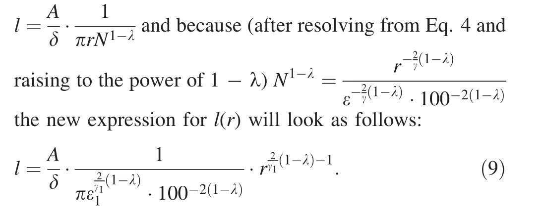
The ratioA/δ may be derived from Eq.8 as πrlN1-λwhere all the terms are supposed to be known.By analogy with Eq.6,there is one unknown term γ1in the exponent and one unknown term ε1in the intercept of Eq.9.Equation 9 obviously generalizes the model because the case of λ =0,which means a flat tendency inSˆ(N),reduces Eq.9to old form of Eq.6.Note that Eq.8 has an impact only onl(r)relationship whiler(N)remains in the old form of Eq.7.

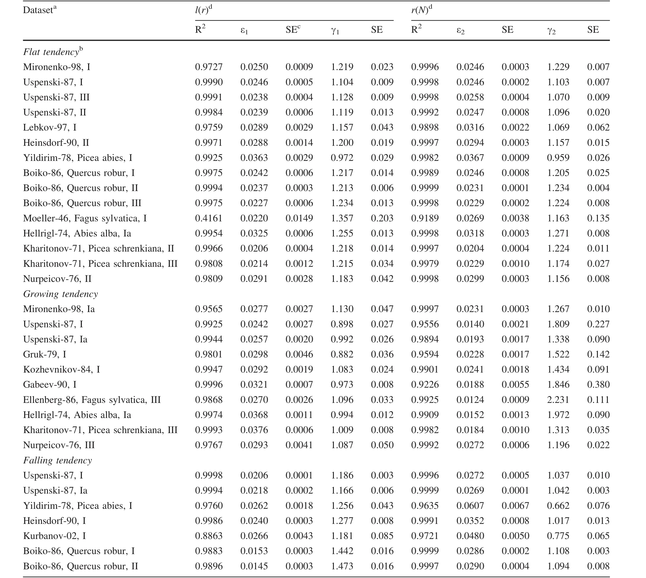
Table 2 Results of computations of parameters ε and γ in relationships l(r)and r(N)

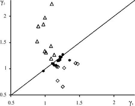
Fig.1 Values ofγ1plotted against γ2foralldatasets.Key: filledcircle datasets with a flat tendency of Sˆ(N)development,open triangle datasets with a growing tendency and diamond datasets with a falling tendency.Straight solid line denotes the position when γ1= γ2

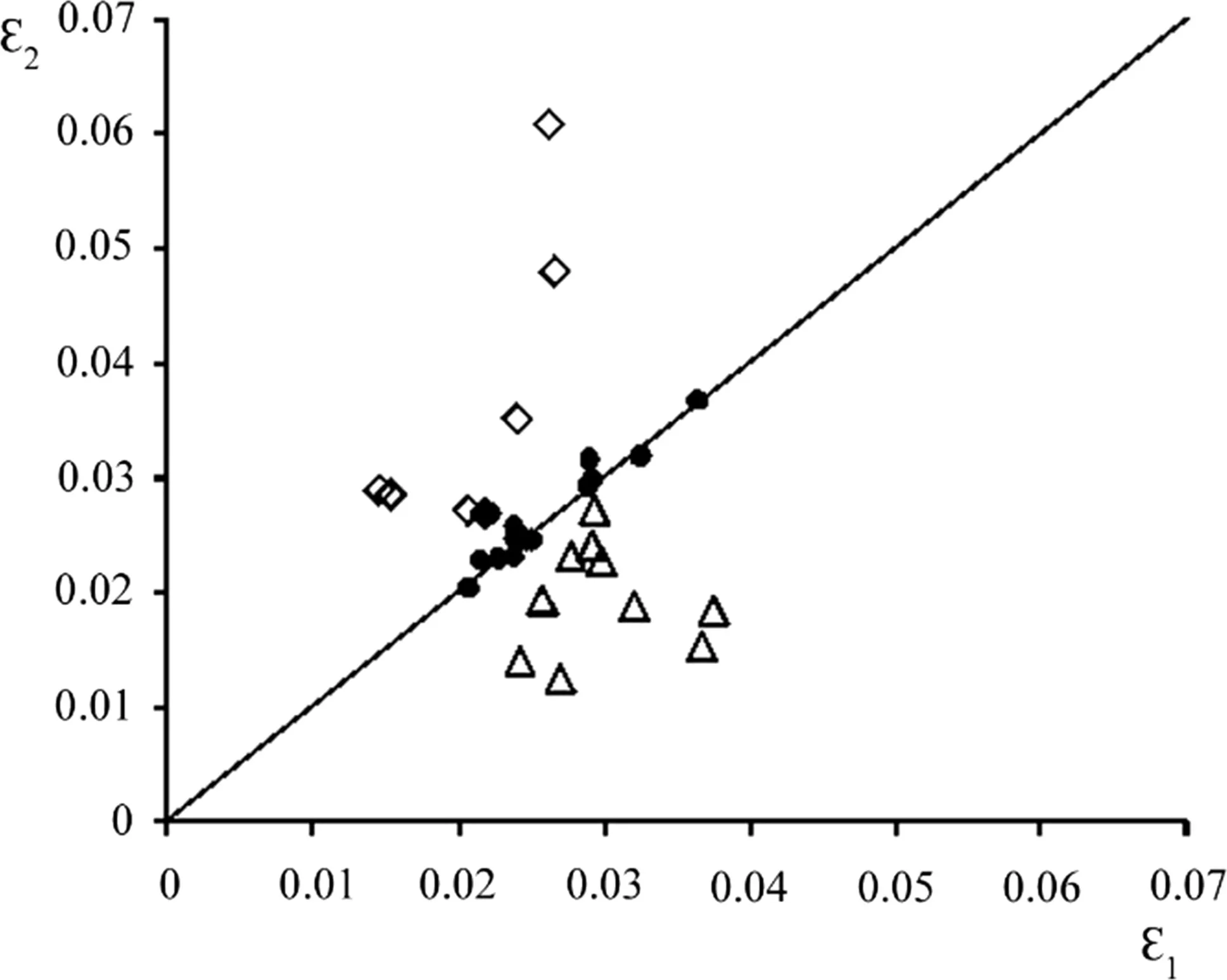
Fig.2 Values of ε1plotted against ε2for all datasets.Legends are same as in Fig.1.Straight solid line denotes the position when ε1= ε2

Again,it is clear that independently estimated ε1(0.0232)and ε2(0.0231)are close to each other.

To summarize,ifSˆ(N)=constant,then exponents inl(r)(Eq.6)andr(N)(Eq.7)are tightly related to each other so that information on one exponent may help to compute the other one.This is done through a common term γ in the exponents.Also,intercepts inl(r)(Eq.6)andr(N)(Eq.7)can be computed from one another through a common term ε.IfSˆ(N) ≠ constant but only a tendency inSˆ(N)is known,then relations between the exponents and intercepts may be estimated in terms of ‘more/less’.

If however,Sˆ(N)may be represented as a power function ofN,i.e.,Sˆ(N)=A·Nλand λ may be quantitatively estimated,then exponents inl(r)(Eq.9)andr(N)(Eq.7)can be readily computed from one another with the help of λ value.The same is true for the intercepts;they can be computed from one another as well.

Conclusion

Numerous relationships have been established in forest science that served to describe structure and growth of forest stands.Some,like the ‘–3/2 self-thinning rule’,were derived from other relations linking sizes of trees to stand density.

In this study,the ‘relationships between relationships’was considered;theHversusDrelationship(height curve)was sought to quantitatively relate to theDversusNrelationship(thinning curve).In order to provide mathematical consistency,all analyzed relations were presented in the form of simple power functions that included an exponent and an intercept.It has been shown that putting hypotheses on how total stem surface area develops during self-thinning or thinning helps to find analytical links between exponents/intercepts of the height curve and exponents/intercepts of the thinning curve.If it is known that total stem surface area does not change in the course of thinning or an exponent is known of the area dependent on stand density,the exponents/intercepts in the relationships may be directly computed from one another.This implies an existence of profound processes that govern the development of a forest stand and this deepens our knowledge on this development.Why such‘relationships between relationships’may appear is a topic of special research,but it may be hypothesized that the source of the phenomenon lies in interactions of trees in the course of growth,competition and dying-off.

AcknowledgementsDr.G.Kofman read the manuscript and made useful suggestions which are gratefully acknowledged.The author thanks two anonymous reviewers who made useful comments that helped to improve the manuscript.

References

Chapman HH(1921)Forest mensuration.Wiley,New York,p 553

Gavrikov VL(2014)A simple theory to link bole surface area,stem density and average tree dimensions in a forest stand.Eur J For Res 133(6):1087–1094.doi:10.1007/s10342-014-0824-4

Gavrikov VL(2015)An application of bole surface growth model:a transitional status of‘-3/2’rule.Eur J For Res 134(4):715–724

Inoue A(2004)Relationships of stem surface area to other stem dimensions for Japanese cedar(Cryptomeria japonicaD.Don)and Japanese cypress(Chamaecyparis obtusaEndl.)trees.J For Res 9(1):45–50

Inoue A(2009)Allometric model of the maximum size–density relationship between stem surface area and stand density.J For Res 14(5):268–275

Inoue A,Nishizono T(2015)Conservation rule of stem surface area:a hypothesis.Eur J For Res 134(4):599–608

Larjavaara M(2010)Maintenance cost,toppling risk and size of trees in a self-thinning stand.J Theor Biol 265(1):63–67

Niklas KJ,Spatz HC(2004)Growth and hydraulic(not mechanical)constraints govern the scaling of tree height and mass.Proc Natl Acad Sci USA 101(44):15661–15663

Pretzsch H(2006)Species-speci fic allometric scaling under selfthinning:evidence from long-term plots in forest stands.Oecologia 146(4):572–583

Pretzsch H,Biber P(2005)A re-evaluation of Reineke’s rule and stand density index.For Sci 51(4):304–320

Reineke LH(1933)Perfecting a stand-density index for even-aged forests.J Agric Res 46(7):627–638

Sterba H(1987)Estimating potential density from thinning experiments and inventory data.For Sci 33(4):1022–1034

Usoltsev VA(2010)Eurasian forest biomass and primary production data.Ural Branch of Russian Academy of Sciences,Yekaterinburg,p 570(in Russian)

van Laar A,Akc¸a A(2007)Forest mensuration.In:Gadow KV,Pukkala T,Tome´M(eds)Managing forest ecosystems,vol 13.Springer,Dordrecht,p 384

Vanclay JK,Sands PJ(2009)Calibrating the self-thinning frontier.For Ecol Manag 259(1):81–85

Yoda K,Kira T,Ogawa H,Hozumi K(1963)Intraspeci fic competition among higher plants.XI.Self-thinning in over-crowded pure stands under cultivated and natural conditions.J Biol Osaka City Univ 14:107–129

Zhang Z,Zhong Q,Niklas KJ,Cai L,Yang Y,Cheng D(2016)A predictive nondestructive model for the covariation of tree height,diameter,and stem volume scaling relationships.Sci Rep 6:31008.doi:10.1038/srep31008