Optimizing Deep Learning Parameters Using Genetic Algorithm for Object Recognition and Robot Grasping

Delowar Hossain, Genci Capi, and Mitsuru Jindai

1.Introduction

Deep learning (DL) starts an upsurge in the artificial intelligence research since Hinton et al.[1]first proposed it. After that, DL has been widely applied in different fields such as complex image recognition, signal recognition, automotive,texture synthesis, military, surveillance, natural language processing, and so on. The main focus of deep architectures is to explain the statistical variations in data and automatically discover the features abstraction from the lower level features to the higher level concepts. The aim is to learn feature hierarchies that are composed of lower level features into higher level features abstraction.

Researches then began on analyzing DL networks for robotics applications. For robotics applications, object recognition is a very crucial research area. Nevita et al.[2]introduced the object recognition process in 1977. After then,researchers had proposed different types of methods for different types of object recognition problems[3]-[7]. Nowadays,DL is gaining popularity in the applications of robotics object recognition. Many researchers have worked on using DL[8]-[13]for several robot tasks. Those contributions make the robot applications useful in industrial applications as well as household work.

However, the DL networks creation and training need significant effort and computation. DL has many parameters that have influenced on the network performance. Recently,researchers are working to integrate evolutionary algorithms with DL in order to optimize the network performance. Young et al.[14]addressed multi-node evolutionary neural networks for DL to automating network selection on computational clusters through hyper-parameter optimization using genetic algorithm(GA). A multilayer DL network using a GA was proposed by Lamos-Sweeney[15]. This method reduced the computational complexity and increased the overall flexibility of the DL algorithm. Lander[16]implemented an evolutionary technique in order to find the optimal abstract features for each auto-encoder and increased the overall quality and abilities of DL. Shao et al.[17]developed an evolutionary learning methodology by using the multi-objective genetic programming to generate domainadaptive global feature descriptors for image classification.

In this paper, we propose the autonomous robot object recognition and grasping system using a GA and deep belief neural network (DBNN) method. GA is applied to optimize the parameters of DBNN method such as the number of epochs,number of hidden units, and learning rates in the hidden layers,which have much influence on the structures of the network and the quality of performance in DL networks. After optimizing the parameters, the objects are recognized by using the DBNN method. Then, the robot generates a trajectory from the initial position to the object grasping position, picks up the object, and places it in a predefined position.

The rest of the paper is organized as follows: DBNN method is described in Section 2; the evolution of DBNN parameters is mentioned in Section 3; the GA evolution results are presented in Section 4; the GA and DBNN implementation on the robot are shown in Section 5. Finally, we conclude the paper and give the future work in Section 6.

2.Methodology

In this paper, we design the robot object recognition and grasping system by successfully applying the DBNN method and GA. The DBNN method is used for object recognition purpose and the GA is used to optimize the DBNN parameters.

2.1　DBNN Method

A DBNN is a generative graphical model composed of stochastic latent variables with multiple hidden layers of units between the input and output layers. A DBNN composes of a stack of restricted Boltzmann machines (RBMs). An RBM consists of a visible layer and a hidden layer or a hidden layer and another hidden layer. The neurons of a layer are fully connected to the neurons of another layer, but the neurons of the same layer are not internally connected with each other. An RBM reaches to the thermal equilibrium when the units of the visible layer are clamped. The general structure of a DBNN method is shown in Fig. 1. The DBNN follows two basic properties: 1) DBNN is a top-down layer-by-layer learning procedure. It has generative weights in the first two hidden layers that would find how the variables in one layer communicate with the variables of another layer, and discriminative weights in the last hidden layer which would be used to classify the objects. 2) After layer-wise learning, the values of the hidden units can be derived by bottom-up pass. It starts from the visible data vector in the bottom layer.

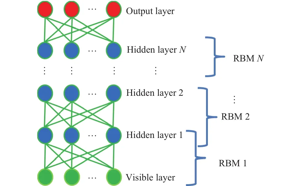
Fig. 1. General structure of a DBNN method.

The energy of the joint configurationbetween visible layer and hidden layer in RBM is with bias values

where v is a set of visible units withand h is a set of hidden units with. nvis the total number of units in the visible layer and nhis the total number of units in the hidden layer. a is the bias term of visible units and b is the bias term of hidden units. w represents the weight between visible units and hidden units.

We apply the DBNN method for object recognition purpose in the proposed experiments. The structures of the proposed implemented DBNN method is shown in Fig. 2. The DBNN method consists of one visible layer, three hidden layers, and one output layer. The visible layer consists of 784 neurons of the input image. The GA[18]finds the optimal number of hidden units in each layer. In our implementation,the number of hidden units in the 1st, 2nd, and 3rd hidden layers are 535, 229, and 355, respectively. The output layer consists of six different types of object classes. In the sampling method, we apply two different types of sampling: Contrastive divergence (CD) and persistent contrastive divergence (PCD).In the first hidden layer, we apply the PCD sampling method,as PCD explores the entire input domain. In the second and third hidden layers, we apply the CD sampling method, as CD explores near the input examples. By combining the two sampling methods, the proposed DBNN method can gather optimal features to recognize objects.

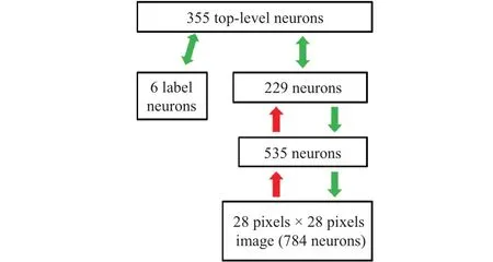
Fig. 2. Structure of the proposed DBNN method.

After training the input features, fine-tuned operation is performed using back propagation in order to reduce the discrepancies between the original data and its reconstruction.We use the softmax function to classify the objects. The back propagation operation will terminate if one of the following conditions is satisfied: 1) reach to the best performance, which is defined by the mean squared error (MSE), 2) reach to the maximum validation check, i.e., 6, 3) reach to the minimum gradient, or 4) reach to the maximum epoch number, i.e., 200.

3.Evolution of DBNN Parameters

Optimization is the process of making the DBNN method better. In the implementation, the aim is to optimize the DBNN parameters in order to improve the performance and the quality of the DL network structures.

In order to optimize the DBNN parameters, we apply an evolutionary algorithm known as GA. A real value parallel GA[18]is employed in our optimization process, which outperforms on the single population GA in terms of the quality of the solution. Using parallel GA, we optimize the number of hidden units, the number of epochs, and the learning rates to reduce the error rate and training time. Our main contributions in parallel GA are the design of the fitness functions and the design of the parameters in the GA structure.

The main goal is to find the optimal number of hidden units, epoch numbers, and learning rates. Therefore, the fitness is evaluated to minimize the error rate and network training time. The fitness function is defined as follows

where eBBP is the number of misclassification divided by the total number of test data before back propagation, eABP is the number of misclassification divided by the total number of test data after back propagation, tBBP is the training time before back propagation, and tDBP is the training time during back propagation operation.

The GA functions and parameters are presented in Table 1.A variety of mutation rates have been tried and the following mutation rates are found to be the best.

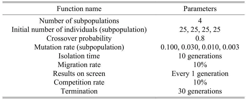
Table 1: GA functions and parameters

4.GA Results

A real value parallel GA has been employed in conjunction with the mutation, selection, and crossover operation. The real value GA performs better comparing with the binary GA. The population size of GA is 100. The best objective value per subpopulation is presented in Fig. 3. It can be seen that the best objective value is 6.54599 on the 24th generation which is shown by red color. The fitness values of each individual through evolution are presented in Fig. 4. In addition, Fig. 4 shows how the number of individuals varies in every subpopulation during evolution. In the initial generation, the fitness value started from 11.5. The worst individuals were removed from the less successful subpopulations. After seven generations, from 50 to 70 in indexes of the individuals, the convergences of the individuals were better. The convergences would be the most successful at the end of the optimization on the 24th generation.

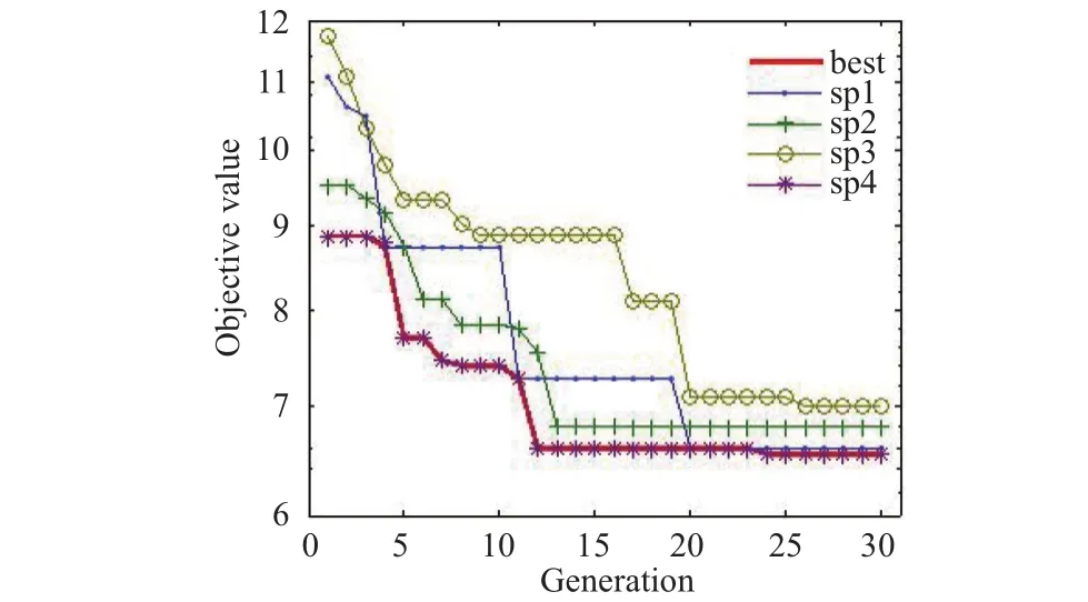
Fig. 3. Best objective values per subpopulation.

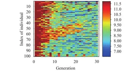
Fig. 4. Fitness value of individuals for all generation.

The performances of GA with arbitrarily selected DBNN parameters were compared in [9]. In the case of arbitrarily selected DBNN parameters, the numbers of hidden units in three hidden layers are 1000, 1000, and 2000, the numbers of epochs are 200, 200, and 200, the learning rate of the 1st hidden layer is 0.001, the learning rates of the 2nd and 3rd hidden layers are both 0.1. In the case of GA, the optimal numbers of hidden units in three hidden layers are 535, 229,and 355, the numbers of epochs are 120, 207, and 221, the learning rate of the 1st hidden layer is 0.04474, the learning rates of the 2nd and 3rd hidden layers are both 0.44727. In both cases, the error rate is nearly same, i.e., 0.0133. The training time has been reduced 84% by using the optimized DBNN parameters compared with the arbitrary DBNN parameters.

5.Experimental Results

5.1　Robot Object Recognition Results

In order to verify the optimized DBNN parameters, the experiments of robot object recognition were considered. A database of six robot graspable objects including four different types of screwdriver, a round ball caster, and a small electric battery was built for the experimental purpose. The database consisted of 1200 images (200 images for each object) in different orientations, positions, and lighting conditions.

At first, the universal serial bus (USB) camera took a snapshot of the experimental environment and this snapshot would be converted to a grayscale image. Then, a morphological structuring element operation was applied in order to detect the existing objects in the environment. The detected objects were separated based on the centroid of the objects in the size of 28 pixels × 28 pixels. Each image was converted to the input vector of 784 neurons by reshaping operation. In addition, normalization and shuffling operations were performed. After then, these input vectors passed through the three hidden layers. As output, the DBNN generates six probability values for each input vector because we train the database using six different types of objects. From this probability values, the objects are recognized. For example, an object image, a red-black screwdriver in this case, is considered as input in Fig. 5. After processing this 28 pixels × 28 pixels image, the input vector passed through three hidden layers. As output, the DBNN generated six probability values including 0.0001, 0.0028, 0.9999, 0.0001, 0.0000, and 0.0000. The highest probability value is 0.9999 which is belonged to the 3rd object. By the same ways, other objects can be recognized.

Fig. 5. Sample object recognition process for a red-black screwdriver.

5.2　Robot Object Grasping Results

For robot object grasping purpose, a PUMA robot manipulator from DENSO Corporation is used. The robot has six degrees of freedom. The robot can grasp any object within the size of 32 mm depth and 68 mm width using the robot gripper. A sequence of experiments for object recognition and robot pick-place operations in different positions, orientations,and lighting conditions were run. The snapshots of the realtime experiments are shown in Fig. 6.

We designed a graphical user interface (GUI). The robot recognized the requested objects using DBNN method when the user required for an intended object by clicking on GUI.The robot found the grasping position based on the object center. The robot generated a trajectory from the initial position to the object grasping position. After reaching to the object position, the robot adjusted its gripper orientation based on the object orientation. Then the robot grasped the intended object,generated another path trajectory to the predefined destination position, placed the object, and returned to the initial position.At the same way, the remaining objects can be recognized and the robot can perform the pick-place operations.

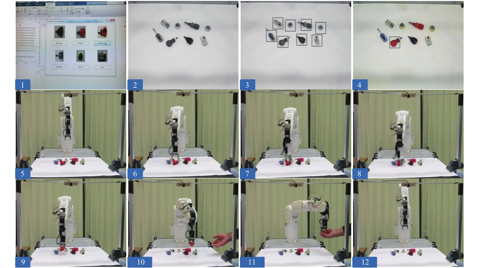
Fig. 6. Snapshots for object recognition and robot grasping process.

6.Conclusions and Future Work

We proposed a GA based DBNN parameters optimization method for robot object recognition and grasping. The proposed method optimized the number of hidden units, the number of epochs, and the learning rates in three hidden layers. We applied the optimized method on the real-time object recognition and robot grasping tasks. The objects were recognized by using the optimized DBNN method, then the robot grasped the objects and placed them in the predefined position. The experimental results show that the proposed method is efficient enough for robot object recognition and grasping tasks.

The most important part of the future work is to integrate multi-population genetic algorithm (MPGA) with DBNN method. Therefore, we plan to investigate the MPGA performance with the different number of subpopulations and other genetic parameters.

[1]G. Hinton, S. Osindero, and Y. W. Teh, “A fast learning algorithm for deep belief nets,”Neural Computation, vol. 18,no. 7, pp. 1527-1554, 2006.

[2]R. Nevita and T. Binford, “Description and recognition of curved objects,”Artificial Intelligence, vol. 8, no. 1, pp. 77-98, 1977.

[3]D. G. Lowe, “Three-dimensional object recognition from single two-dimensional images,”Artificial Intelligence, vol.33, no. 1, pp. 355-395, 1987.

[4]M. Lades, J. C. Vorbruggen, J. Buhmannet al., “Distortion invariant object recognition in the dynamic link architecture,”IEEE Trans. on Computers, vol. 42, no. 3, pp.300-311, 1993.

[5]J. R. R. Uijlings, K. E. A. V. D. Sande, T. Gevers, and A. W.M. Smeulders, “Selective search for object recognition,”Intl.Journal of Computer Vision, vol. 104, no. 2, pp. 154-171,2013.

[6]P. Agrawal, R. Girshick, and J. Malik, “Analyzing the performance of multilayer neural networks for object recognition,” inProc. of European Conf. on Computer Vision, 2014, pp. 329-344.

[7]P. Wohlhart and V. Lepeti, “Learning descriptors for object recognition and 3D pose estimation,” inProc. of IEEE Conf.on Computer Vision and Pattern Recognition, 2015, pp.3109-3118.

[8]D. Hossain and G. Capi, “Application of deep belief neural network for robot object recognition and grasping,” inProc.of the 2nd IEEE Intl. Workshop on Sensing, Actuation, and Motion Control, 2016, pp. 1-4.

[9]D. Hossain, G. Capi, and M. Jindai, “Object recognition and robot grasping: A deep learning based approach,” inProc. of the 34th Annual Conf. of the Robotics Society of Japan,2016, pp. 1-4.

[10]I. Lenz, H. Lee, and A. Saxena, “Deep learning for detecting robotic grasps,”Intl. Journal of Robotics Research, vol. 34,no. 4-5, pp. 705-724, 2013.

[11]L. Pinto and A. Gupta, “Supersizing self-supervision:Learning to grasp from 50K tries and 700 robot hours,” inProc. of IEEE Intl. Conf. on Robotics and Automation, 2016,pp. 16-21.

[12]J. Redmon and A. Angelova, “Real-time grasp detection using convolutional neural networks,” inProc. of IEEE Intl.Conf. on Robotics and Automation, 2015, pp. 1316-1322.

[13]S. Levine, P. Pastor, A. Krizhevsky, and D. Quillen,“Learning hand-eye coordination for robotic grasping with deep learning and large-scale data collection,” inProc. of Intl. Symposium on Experimental Robotics, 2016, pp. 173-184.

[14]S. Young, D. Rose, T. Karnowski, S. Lim, and R. Patton,“Optimizing deep learning hyper-parameters through an evolutionary algorithm,” inProc. of the Workshop on MachineLearninginHigh-PerformanceComputing Environments, 2015, pp. 4:1-18.

[15]J. Lamos-Sweeney, “Deep learning using genetic algorithms,” M.S. thesis, Dept. Rochester Institute of Technology, NY, USA, 2012.

[16]S. Lander, “An evolutionary method for training auto encoders for deep learning networks,” M.S. thesis, Dept.Computer Science, Missouri Univ., USA, 2014.

[17]L. Shao, L. Liu, and X. Li, “Feature learning for image classification via multi-objective genetic programming,”IEEE Trans. on Neural Networks and Learning Systems, vol.25, no. 7, pp. 1359-1371, 2014.

[18]G. Capi and K. Doya, “Evolution of recurrent neural controllers using an extended parallel genetic algorithm,”Robotics and Autonomous System, vol. 52, no. 2-3, pp. 148-159, 2005.