Approximate Solution of the Kuramoto-Shivashinsky Equation on an Unbounded Domain∗

Wael W.MOHAMMED

1 Introduction

In this paper,we are interested in the long time behaviour of nonlinear parabolic partial differential equations(PDEs for short)defined on unbounded domain near its change of stability.First aim here is to derive rigorously the modulation equation of

in the following type

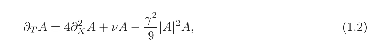
where L in(1.1)is the linear differential operator−(1−k2)2for k∈R and corresponding to eigenfunctions eikx.

Second aim of this paper is to approximate the solution ψ of(1.1)by

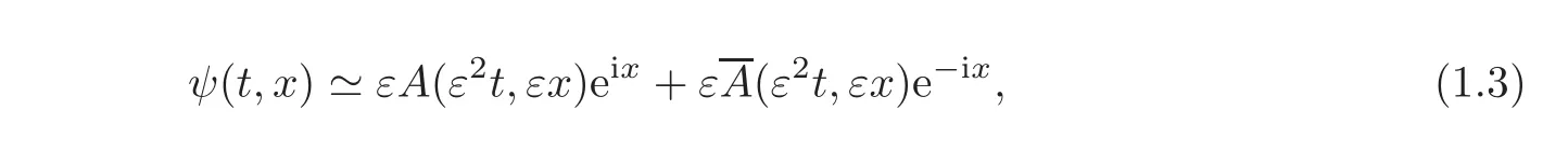
where A(T,X)is the solution of the G-L equation(1.2)with T= ε2t and X= εx.

The Kuramoto-Sivashinsky(K-S for short)equation(1.1)was proposed in the year 1977 by Kuramoto[11]as a model for phase turbulence in reaction diffusion systems.The equationwas also developed by Sivashinsky[22]in higher space dimensions in modelling small thermal diffusive instabilities in Laminar flame fronts.

The K-S equation arises in many physical problems includingflame front instabilities and reaction-diffusion combustion dynamics(see[22–23]),propagation of concentration waves in chemical physics applications(see[11–13]),and falling film flows(see[7,10,24]).

Different approaches have been proposed in literature to investigate and seek the solutions of the K-S equation.Some of these methods are variational iteration methods(see[19]),the lattice Boltzmann technique(see[14]),the tanh function method(see[5]),the method of radial basis functions(see[9]),the local discontinuous Galerkin method(see[25]),Perturbation methods(see[20,26]),the Chebyshev spectral collocation scheme(see[3]).Recently,there are other various methods that have also been developed to construct exact solutions of the K-S equation(see[4,6,27–28]).

Ma and Fuchssteiner[15]used the perturbation method and considered approximate solutions to obtain a complete integrable system.On the other hand,Schneider[20]used the perturbation method and approximated the solution of the K-S equation(1.1)on an unbounded domain via the solution of the G-L equation(1.2).But Schneider’s method relies on the high regularity of the modulation equation,as he needed

Mielke and Schneider[16]compared the long-time behaviour of all solutions of equation(1.1)with the long-time behaviour of the solution A of(1.2),and they discussed the question of how the attractor can be described by the attractor of the G-L equation(1.2).For this case,similar results are well known(see for instance[8,17,21]).

In this paper,we use the perturbation method to approximate the solutions of the KS equation(1.1).This method depends on the low regularity of the modulation equation.Unfortunately,some regularity for A is needed.So A must be in([0,T],H12+).

We will prove the following approximation result for the K-S equation(1.1)via the G-L equation(1.2).

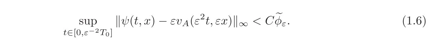
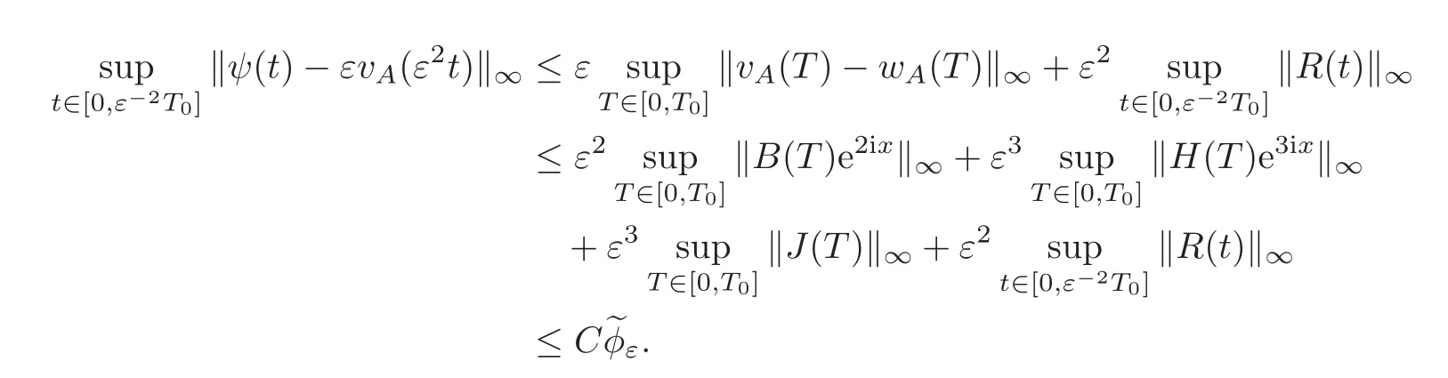
Theorem 1.1Letψ(t,x)be a solution of the K-S equation(1.1),vA(T,X)be the formal approximation defined as

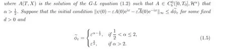
Then,for eachT0＞0there exists a constantC＞0,depending

The rest of this paper is organized as follows.In next section,we give a formal derivation of the modulation equation.In Section 3,we define Hαand give the relation between the norm in Hαand the norm in(R).In Section 4,we define the Green’s function Gt(x)and give estimates on it.Finally,Section 5 is devoted to the proof of the approximation theorem.

2 Formal Derivation of the Modulation Equation

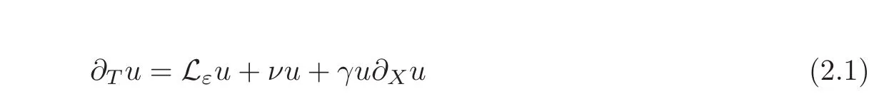
This section is devoted to derive the modulation equation corresponding to equation(1.1).Let usfirst rescale the equation(1.1).If

then(1.1)becomes

Now,let

where the amplitudes A,B,M,H,J are functions of T and X and c.c.denotes the complex conjugation of the terms preceding it within the brackets.By plugging(2.2)into(2.1)and using the relation

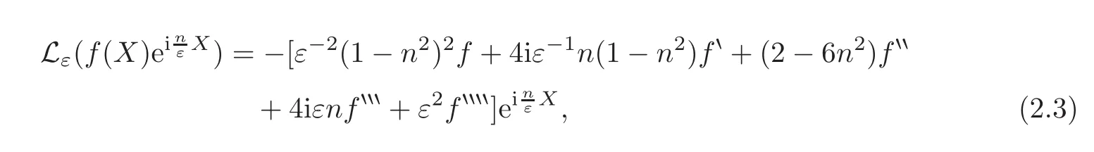
yields

In order to remove all unwanted terms,let

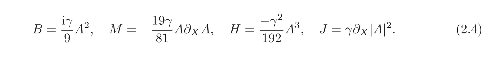
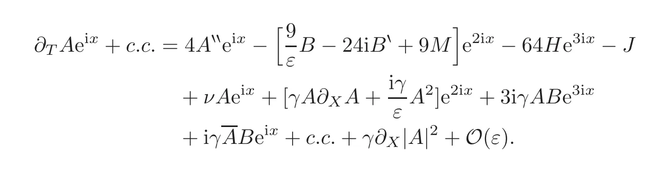
Hence,

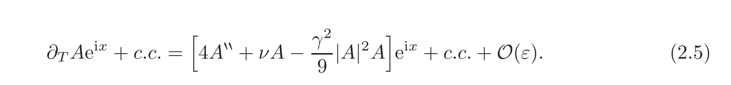
By equating the coefficients terms of eixin(2.5),we obtain

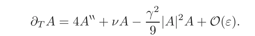
By neglecting all small terms in ε,we obtain(1.2).

3 The Hα-Spaces

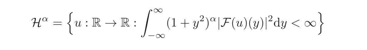
We start this section by giving the definition of the fractional Sobolev space Hα.We rely in this definition on weighted L2-norms of Fourier transforms.

Definition 3.1Forα ∈ R.The spaceHαis defined as

with norm

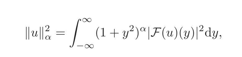
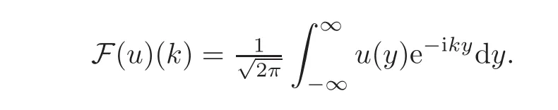
whereF(u)is the Fourier transform ofu,defined by

Note that functions still decay to 0 at∞ in the space Hα.So if A∈Hα,then the solutions of(1.1)and the solutions of(1.2)still decay to 0 as|x|tends to∞.

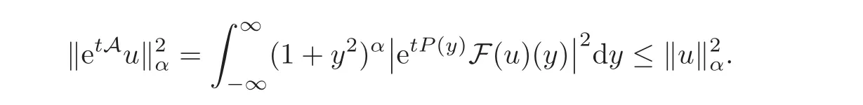
Lemma 3.1LetP(k)≤0be the eigenvalues of the non-positive operatorA,whereF(Au)=P(·)F(u).Then fort≥ 0andu ∈ Hα,

It is well known that etA,defined by F(etAu)=etPF(u),generates a contraction semigroup.

ProofFrom Definition 3.1,we note that(as e2tP(k)≤ 1)

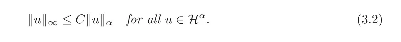
The following lemma gives the relation between the norm in Hαand the norm in(R).For the proof see[2]or Theorem 5.4 in[1].

Lemma 3.2Forα ＞,there is a constantC＞0,such that

To estimate the nonlinearity,we need the following lemma which states that the space Hαis up to the constant a Banach algebra for α ＞.For the proof,see Theorem 4 in[18].

Lemma 3.3Forα＞andm∈N,there exists a positive constantC,such that

In the proof we will need to following generalization of Gronwall’s lemma.

Lemma 3.4Leta,b≥ 0,0≤ ρ,η ＜ 1and0＜ T ＜ ∞.Then,there exists a constantM=M(a,b,η,T),such that for all integrable functionsu:[0,T]→ Rsatisfying

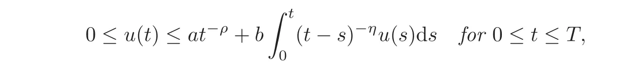
it follows that

4 Semigroup and Green’s Function Estimation

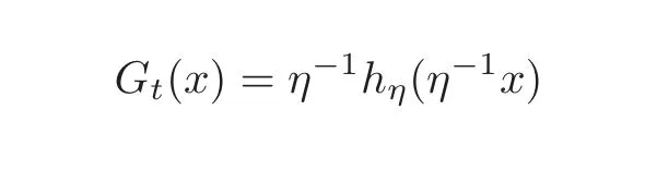
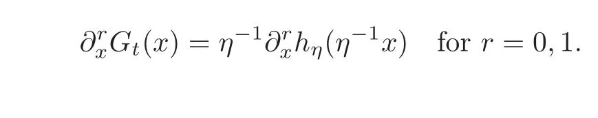
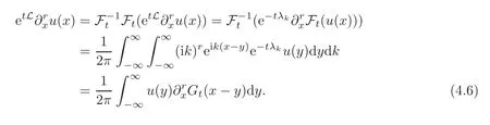
In this section,we give the definition of the Green’s functions Gt(x)for the operator L.Then,we give estimates on it,where we follow the ideas of Collet and Eckmann[8],but for a different operator.Now,we define the Green’s functions Gt(x)as follows.

Definition 4.1DefineGt(x)as

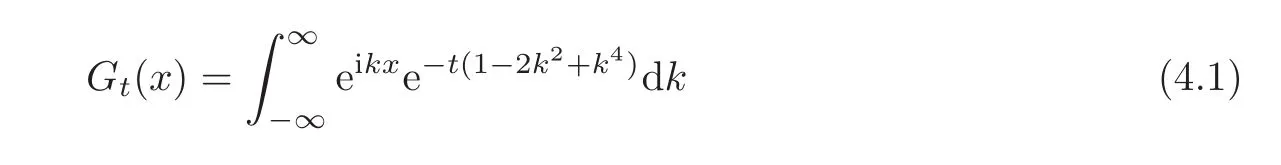
fort＞0.

It is easy to verify that for the semigroup we have

The next lemma states that Gt(x)is bounded regards to ‖ ·‖L1.

Lemma 4.1Lett＞0.Then there exists a positive constantCsuch that

Before we complete the proof of this lemma,we state and prove the next two lemmas.

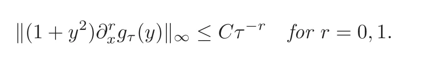
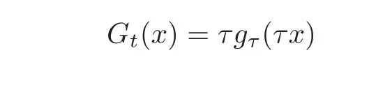
Lemma 4.2Definegτ(y)as

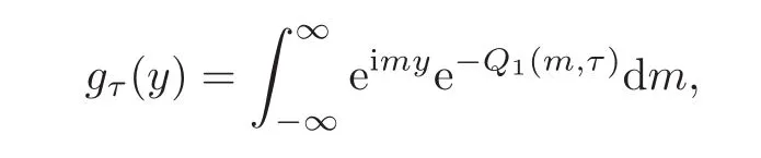
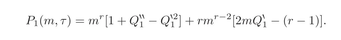
whereQ1(m,τ)= τ−2−2m2+τ2m4,then for0＜ τ≤ 1,there exists a constantC ＞ 0,such that

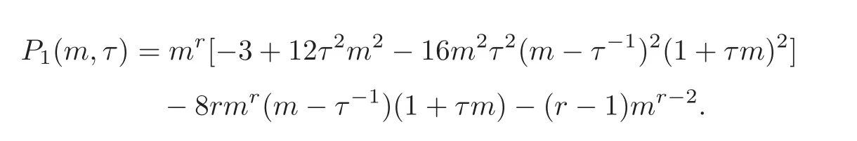
ProofBy using integration by parts,we obtain

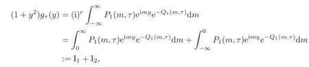
where

We note,for m≥0 and 0＜τ≤1,that

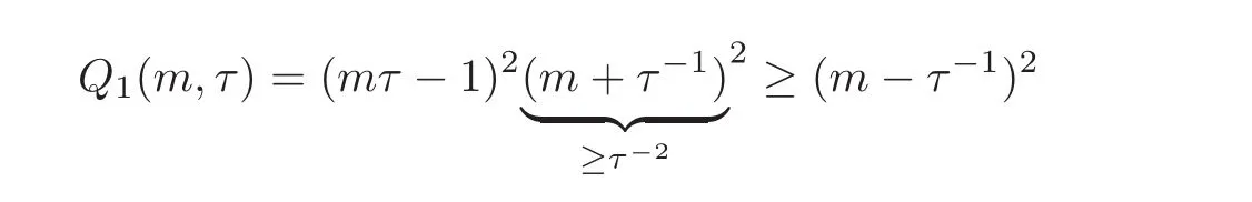
and

Thus

Now we bound I1and I2separately.For thefirst integral I1,we obtain

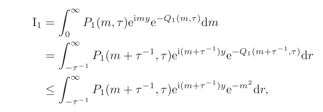
where we used the substitution m=m − τ−1,thus

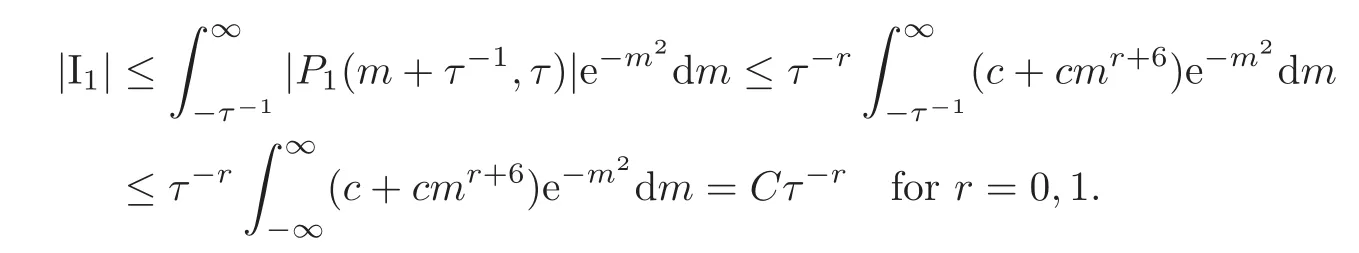
For the second integral I2.By replacing m by−m,we obtain

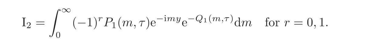
Analogously for thefirst integral,we derive

Hence for 0＜τ≤1,we obtain

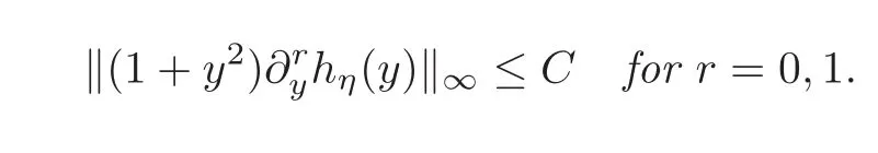
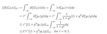
Lemma 4.3Definehη(y)as

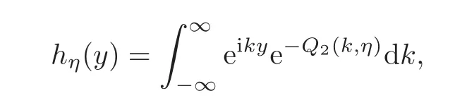
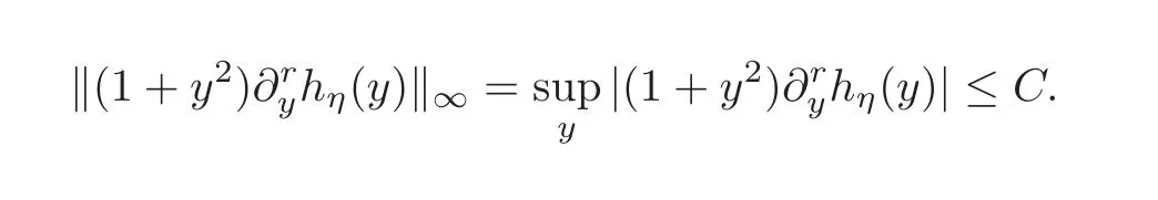
whereQ2(k,η)= η4−2η2k2+k4,then for0＜ η ＜ 1,there exists a constantC ＞ 0,such that

ProofBy using integration by parts,we obtain

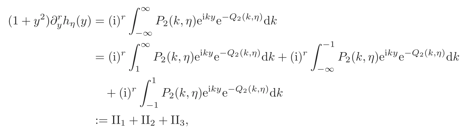
where

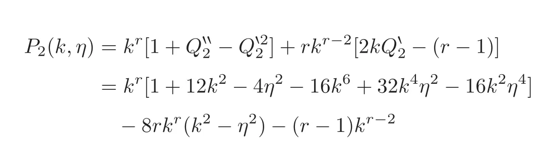
for r=0,1.We note for 0＜η＜1 and k≥1 that

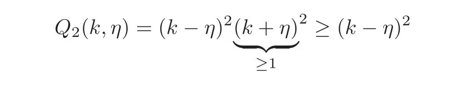
and

Now,We will bound the terms II1,II2and II3separately.To bound II1and II2,we follow the same steps as in the case of Lemma 4.2.To bound the third term:

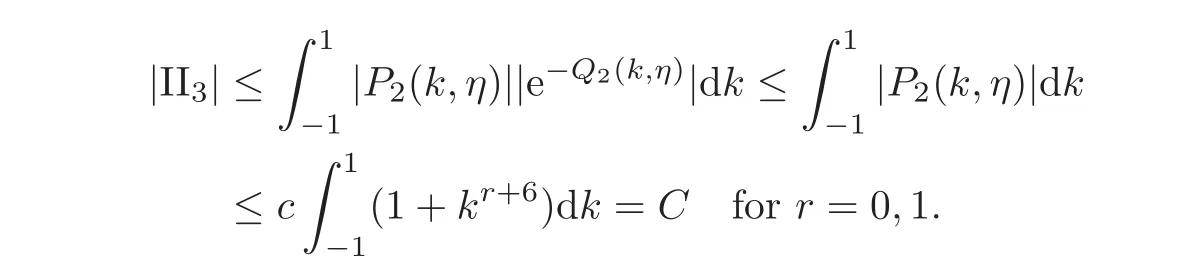
Hence for 0＜η＜1,we obtain,for r=0,1,

Proof of Lemma 4.1We consider two cases in order to prove(4.2).

Case 1t≥ 1:We note for τ=t−12that

and

Hence

where y= τx.By using Lemma 4.2,we obtain for t≥ 1,

Case 2t∈ (0,1):We note for η=t1

4that

and

Hence,

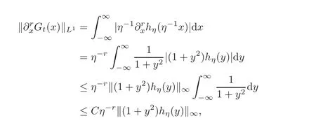
where y= ηx.By using Lemma 4.3,we have for t∈ (0,1),

Combining(4.3)and(4.4),yields(4.2)for t＞0.

Lemma 4.4Fort≥0,there is a constantC＞0,such that

ProofLetdenote the inverse Fourier transform.Then,

Thus

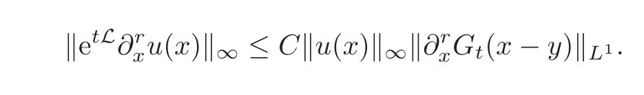
Using Lemma 4.1,yields(4.5).

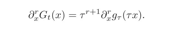
Corollary 4.1ForT≥0,there is a positive constantC,such that

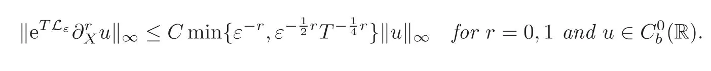
Proof

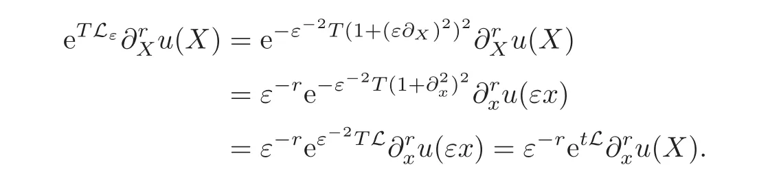
By using Lemma 4.4,we get for r=0,1,

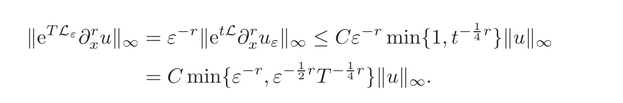
The next lemma allows us to replace the semigroup eTLεby the semigroup e4T∂2X,when they are applied to Aeiε−1X.

Lemma 4.5ForT＞0andA∈Hαwithα＞there is a positive constantC,such that

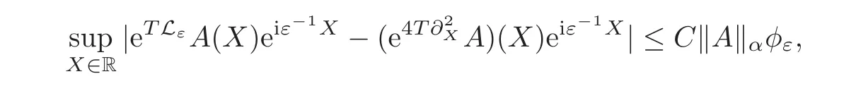
whereφεis defined as

ProofWe can write etLA(εx)eixas a convolution with the Green’s function of L,as in(4.6),

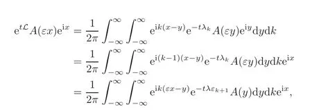
where we used the substitution k= ε−1(k −1)and y= εy.Hence,

where we used|e−4εTk3|≤ 1 for all k ≥ 0 for the first integral and −2k2(2εk+1)≤ 0 for the second integral.Analogously,we can write(e4t∂2xA)(εx)eixas

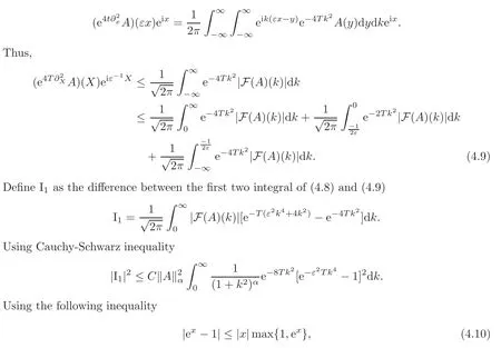
which follows directly from the intermediate value theorem,in order to obtain

Now,we can use the fact

to get

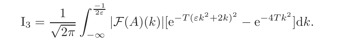
Analogously,we define I2as the difference between the second two integral of(4.8)and(4.9)in order to obtain

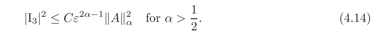
Now,define I3as the difference between the second two integral of(4.8)and(4.9)

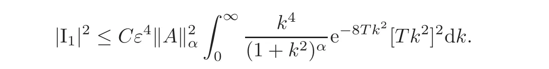
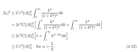
Using Cauchy-Schwarz inequality

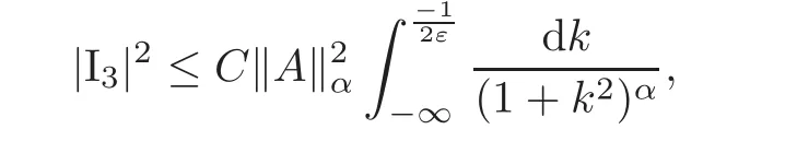
where we used|e−T(εk2+2k)2− e−4Tk2|2 ≤ 2|e−T(εk2+2k)2|2+2|e−4Tk2|2 ≤ 4.Thus

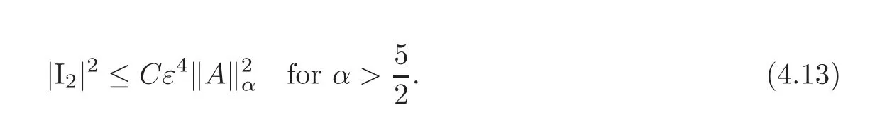
Now

We finish the proof by taking|·|on both sides of(4.15)and using(4.12)–(4.14).

Lemma 4.6Letn∈R{±1}andr∈{0,1}.IfT＞0andM ∈Hα,∀α＞,then there exists a positive constantC,such that

where

ProofWriting etLM(εx)einxas

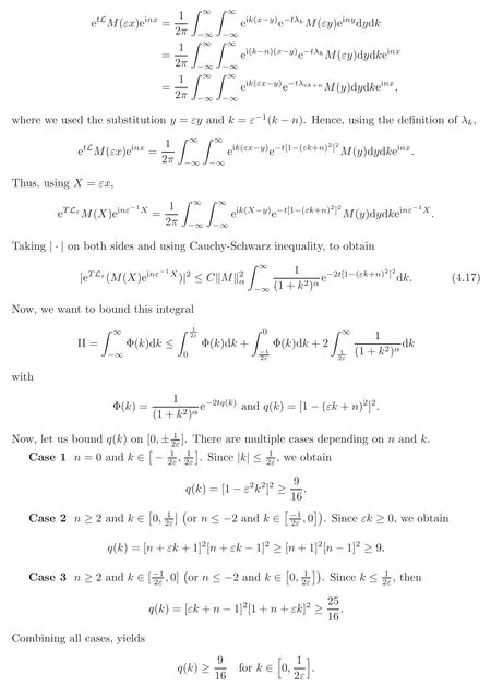
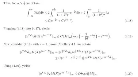
Wefinish the proof by collecting(4.19)and(4.20).

5 Proof of the Approximation Theorem

We present in this section the proof of the approximation theorem.

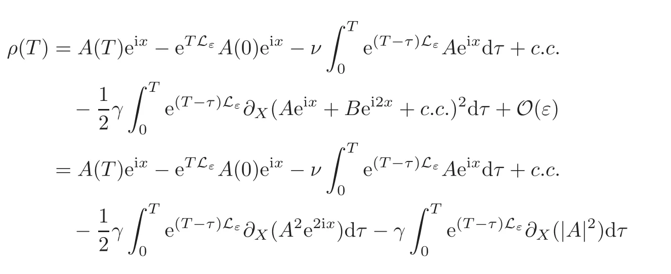
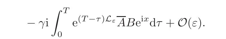
Definition 5.1Define the residualρ(T)as

wherewAis defined in(2.2).

Lemma 5.1

whereis defined in(1.5).

ProofWe obtain from(1.4)

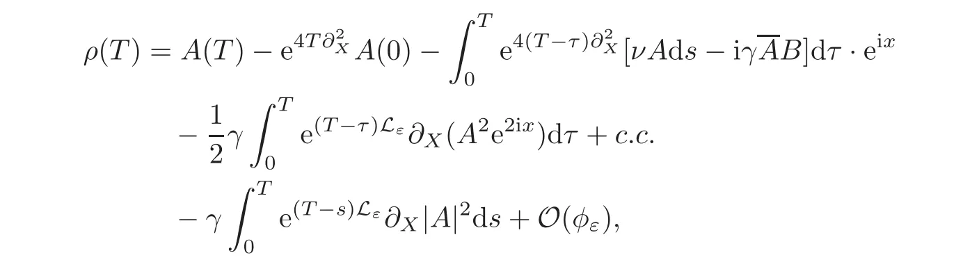
where φεis defined in(4.7)from(1.2),we have

Taking‖·‖∞on both sides and using Lemma 4.6 to get

In the end,we use the results previously obtained to prove the approximation Theorem 1.1 for the solution of the Kuramoto-Shivashinsky equation(1.1).

Proof of the Approximation Theorem 1.1Using multiplier theorem to separate the critical and non critical modes in Fourier space by so called the modefilters.Fix 0＜σ≤Let χ be acut offfunction with

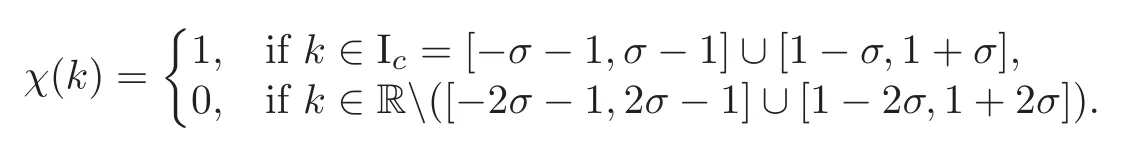
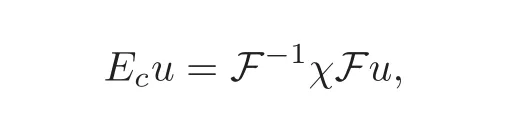
Then,we define the mode filter for the critical modes by

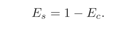
and for the stable modes by

Since Ecand Esare not projections,we define auxiliary mode filters Pcand Pssatisfying PcEc=Ecand PsEs=Esby

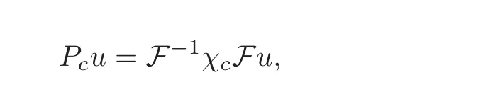
where χcis acut offfunction defined as

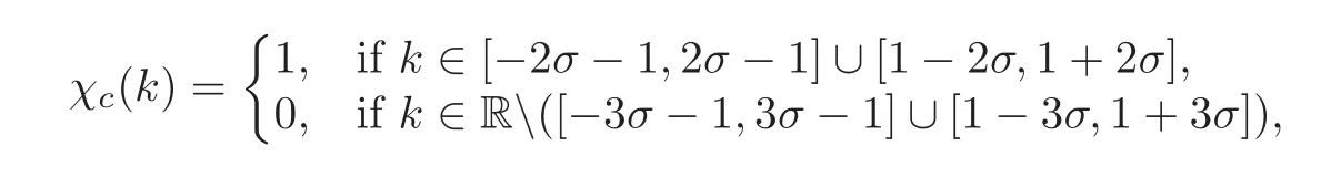
and by

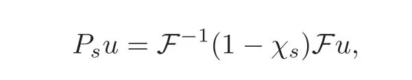
where χsis acut offfunction defined as

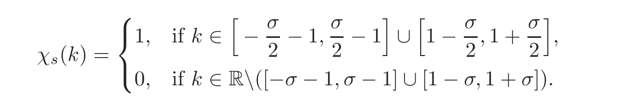
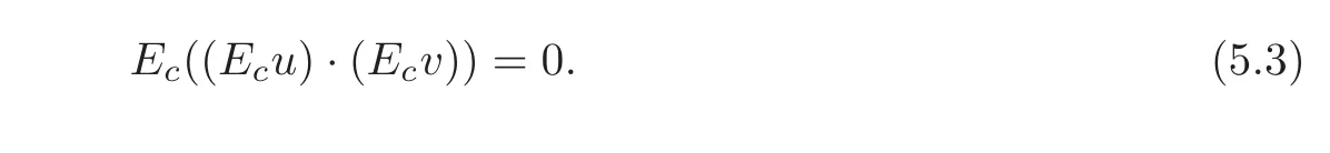
Hence,due to disjoint supports in Fourier space,we can use that

Now define

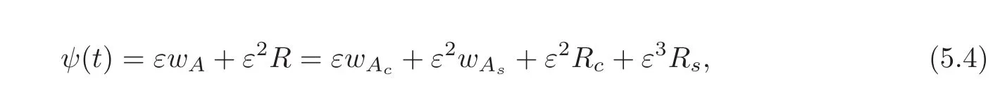
where wAc=EcwA,wAs=EswA,Rc=EcR and Rs=EsR,for short.

Substituting(5.4)into(1.1),we obtain

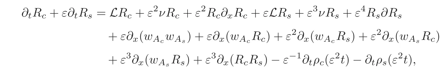
where ρ(T)is defined in(5.1)and ρc=Ecρ,ρs=Esρ.

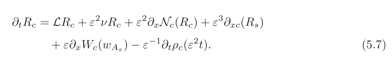
Applying the operators Pcand Ps,we obtain the following system

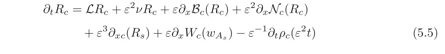
and

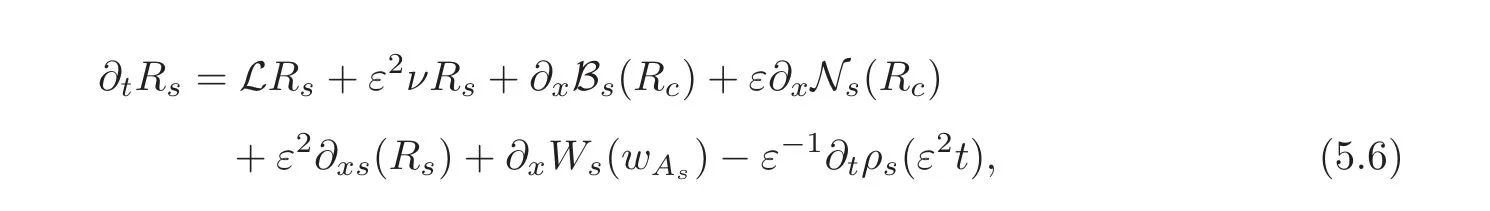
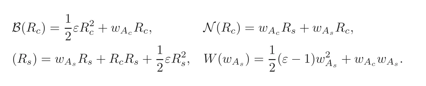
where

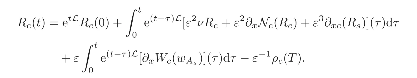
Applying Ecinto both sides of(5.5)and using(5.3),yields

Integrating from 0 to t,we obtain

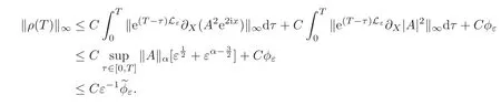
Taking ‖·‖∞on both sides and using Lemma 3.1,yields

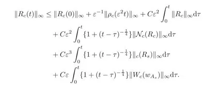
It is easy to bound Nc(Rc),c(Rs)and Wc(wAs)as follows

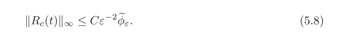
Thus,by using Lemma 3.4(Gronwall’s lemma)with‖Rc(0)‖∞,we obtain

Analogously,for(5.6)we obtain

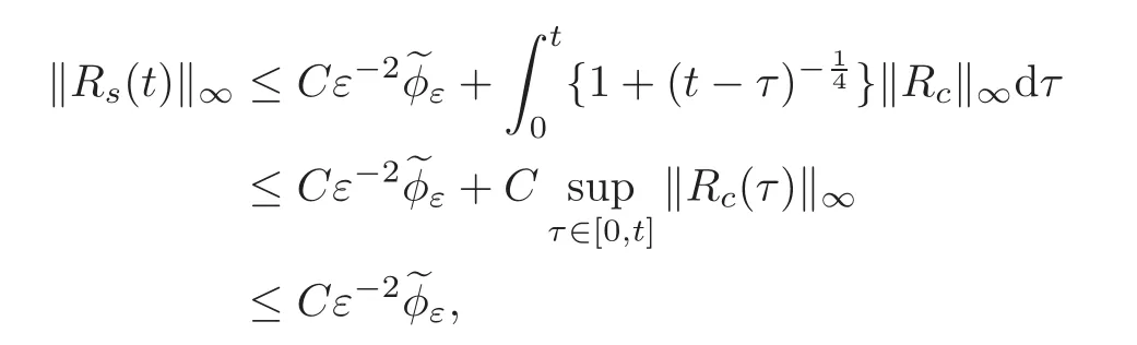
where we used(5.8).Hence,

Since

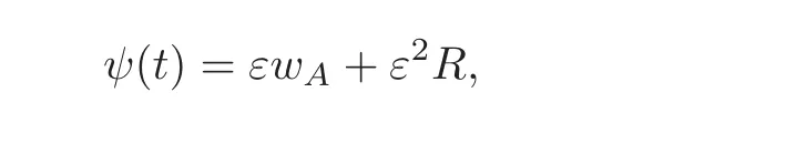
we have

AcknowledgementThe authors would like to express their sincere thanks to the referees for helpful suggestions.

[1]Adams,R.A.,Sobolev spaces,Academic Press,New York,1975.

[2]Adams,D.R.and Hedberg,L.I.,Function Spaces and Potential Theory,Springer-Verlag,1996.

[3]Adomian,G.,Solving Frontier Problems of Physics:The Decomposition Method,Kluwer Academic Publishers,Boston and London,1994.

[4]Alizadeh-Pahlavan,A.,Aliakbar,V.,Vakili-Farahani,F.and Sadeghy,K.,MHD flows of UCM fluids above porous stretching sheets using two-auxiliary-parameter homotopy analysis method,Commun.Nonlinear Sci.Numer.Simul.,14,2009,47388.

[5]Awrejcewicz,J.,Andrianov,I.V.and Manevitch,L.I.,Asymptotic Approaches in Nonlinear Dynamics,Springer-Verlag,Berlin,1998.

[6]Baldwin,D.,Goktas,O.,Hereman,W.,et al.,Symbolic computation of exact solutions expressible in hyperbolic and elliptic functions for nonlinear PDEs,J.Symbolic Comput.,37,2004,669–705.

[7]Benney,D.J.,Long waves on liquid films,J.Math.Phys.,45,1966,150–155.

[8]Collet,P.and Eckmann,J.P.,The time dependent amplitude equation for the Swift-Hohenberg problem,Comm.Math.Physics.,132,1990,139–153.

[9]He,J.H.,Homotopy perturbation technique,Comput.Meth.Appl.Mech.Eng.,178,1999,25762.

[10]Hooper,A.P.and Grimshaw,R.,Nonlinear instability at the interface between twofluids,Phys.Fluids,28,1985,37–45.

[11]Kuramoto,Y.,Diffusion-induced chaos in reaction systems,Suppl.Prog.Theor.Phys,64,1978,346–367.

[12]Kuramoto,Y.and Tsuzuki,T.,On the formation of dissipative structures in reaction diffusion systems,Prog.Theor.Phys.,54,1975,687–699.

[13]Kuramoto,Y.and Tsuzuki,T.,Persistent propogation of concentration waves in dissipative media far from thermal equilibrium,Prog.Theor.Phys.,55,1976,356–369.

[14]Liao,S.J.,A kind of approximate solution technique which does not depend upon small parameters(II):An application influid mechanics,Int.J.Nonlinear Mech.,32(8),1997,1522.

[15]Ma,W.X.and Fuchssteiner,B.,Integrable theory of the perturbation equations,Chaos,Solitons&Fractals,7(8),1996,1227–1250.

[16]Mielke,A.and Schneider,G.,Attractors for modulation equations on unbounded domains-existence and comparison,Nonlinearity,8,1995,743–768.

[17]Mielke,A.,Schneider,G.and Ziegra,A.,Comparison of inertial manifolds and application to modulated systems,Math.Nachr.,214,2000,53–69.

[18]Runst,T.and Sickel,W.,Sobolev Spaces of Fractional Order,Nemytskij Operators,and Nonlinear Partial Differential Equations,Walter de Gruyter,Berlin,New York,1996.

[19]Sajid,M.,Hayat,T.,Comparison of HAM and HPM methods for nonlinear heat conduction and convection equations,Nonlinear Anal:Real World Appl.,9,2008,2296301.

[20]Schneider,G.,A new estamite for the Ginzburg-Landau approximation on the real axis,J.Nonlinear Science,4,1994,23–34.

[21]Schneider,G.,The validity of generalized Ginzburg-Landau equations,Math.Methods Appl.Sci.,19(9),1996,717–736.

[22]Sivashinsky,G.I.,Nonlinear analysis of hydrodynamic instability in laminarflames I:Derivation of basic equations,Acta Astronau,4,1977,1177–1206.

[23]Sivashinsky,G.I.,Instabilities,pattern formation,and turbulence inflames,Annu.Rev.Fluid Mech.,15,1983,179–199.

[24]Shlang,T.and Sivashinsky,G.I.,Irregularflow of a liquid film down a vertical column,J.Phys.,43,1982,459–466.

[25]Van Gorder,R.A.and Vajravelu,R.A.,Analytic and numerical solutions to the Lane-Emden equation,Phys.Lett.A,372,2008,60605.

[26]Von Dyke,M.,Perturbation Methods in Fluid Mechanics,The Parabolic Press,Stanford,California,1975.

[27]Yabushita,K.,Yamashita,M.and Tsuboi,K.,An analytic solution of projectile motion with the quadratic resistance law using the homotopy analysis method,J.Phys.A,40,2007,840316.

[28]Zhu,S.P.,A closed-form analytical solution for the valuation of convertible bonds with constant dividend yield,ANZIAM J.,47,2006,47794.