Experimental investigation of control updating period monitoring in industrial PLC-based fast MPC:Application to the constrained control of a cryogenic refrigerator

Fran¸cois BONNE,Mazen ALAMIR,Patrick BONNAY

1.Universite Grenoble Alpes,INAC-SBT,F-38000 Grenoble,France;

2.CNRS,Gipsa-lab,Universite Grenoble Alpes,F-3800 Grenoble,France

Experimental investigation of control updating period monitoring in industrial PLC-based fast MPC:Application to the constrained control of a cryogenic refrigerator

Fran¸cois BONNE1,Mazen ALAMIR2†,Patrick BONNAY1

1.Universite Grenoble Alpes,INAC-SBT,F-38000 Grenoble,France;

2.CNRS,Gipsa-lab,Universite Grenoble Alpes,F-3800 Grenoble,France

In this paper,a complete industrial validation of a recently published scheme for on-line adaptation of the control updating period in model predictive control is proposed.The industrial process that serves in the validation is a cryogenic refrigerator that is used to cool the supra-conductors involved in particle accelerators or experimental nuclear reactors.Two recently predicted features are validated:the first states that it is sometimes better to use less efficient(per iteration)optimizer if the lack of efficiency is over-compensated by an increase in the updating control frequency.The second is that for a given solver,it is worth monitoring the control updating period based on the on-line measured behavior of the cost function.

Fast MPC,cryogenic refrigerators,control updating period,ODE-based optimization

1 Introduction

Model predictive control (MPC) is an attractive control design methodology because it offers a natural way to express optimal objective while handling constraints on both state and control variables [1]. MPC design is based on the repetitive on-line solution of finite-horizon openloop optimal control problems that are parametrized by the state value.Once the optimal sequence of control inputs is obtained,the first control in the sequence is applied over some updating period τuduring which,the new problem(based on the next predicted state)is solved and the resulted solution is applied while the prediction horizon is shifted by τutime units and the process is repeated yielding an implicit state feedback.

The attractive features of MPC triggered attempts to apply it to increasingly fast systems.For such systems,the need for a high updating rate(small τu)may be incompatible with a complete solution of the underlying optimization problem during a single updating period τu.This fact fired a rich and still active research area that is shortly referred to by “Fast MPC”(see[2–5]and the reference therein).

Typical issues that are addressed in fast MPC literature concern the derivation of efficient computation of updating steps,reduction of the feedback delay,more or less rigorous computation of the Hessian,etc.Typical proofs of closed-loop stability in that context(see for instance[5])depend on strong assumptions such as the proximity to the optimal solution,the quality of the Hessian matrix estimation,etc.With such assumptions,the corresponding stability proofs take the form of tautological assertions.In other words,when such assumptions are satisfied,the paradigm of fast MPC is less relevant since standard execution of efficient optimizers would anyway give satisfactory results.

When the effectively applied control is far from being optimal(which is the case for instance after a sudden change in the set-point value)the hot-start(initialization of the decision variable after horizon shift)it induces for the next horizon does not necessarily decrease the cost function before several iterations.This is because far from the ideal solution,the final stabilizing constraints invoked in the formal proof of[1]may be far from being satisfied.On the other hand,if a constant large control updating period is used in order to accommodate for such situations,the overall closed-loop performance would be badly affected.

In recent papers[6,7],investigations have been conducted regarding the impact of the choice of the control updating period τuon the behavior of the cost function.Simple algorithms have been also proposed to monitor on-line the updating period based on the on-line behavior of the cost function to be decreased.More recently[8,9],it has been shown that the control updating period choice is intimately linked to the basic iteration being used.The two major facts that come out from these investigations can be summarized as follows:

Fact 1In a constant updating period schemes and under computation power constraints,the computation time of the solver algorithm is a priority compared to its efficiency(per iteration)[8].This fact enhanced the recent interest[10,11]in fast gradient-like algorithms[12]as a simpler approach when compared to second order algorithms.The work in[8]gives a formal explanation for this intuitively accepted fact.

Fact 2For a given optimization algorithm,the closed-loop performance can be enhanced by a quasi computation-free on-line adaptation rule of the control updating period[6,7].

Obviously,a combination of the preceding facts holds also,namely,in adaptive frameworks,it can be more efficient to use simpler optimization algorithms provided that the gain induced by a higher updating rate compensates for the lack of efficiency per iteration.

In view of the preceding discussion,the contribution of this paper is twofold:

First contributionThis paper gives the first industrial validation of the proposed on-line adaptation of the control updating period.The realistic PLC-based implementation framework being used enhances the sensitivity of the closed-loop performance to the adaptation mechanism since it is several orders of magnitude slower than nowadays desk computers. As such, this paper gives a complete and realistic layout to understand the chain of concepts and methods that underline fast MPC paradigm.

Second contributionAlthough simulation-based assessments have been proposed for Facts 1 and 2 mentioned above,these simulations always used first order gradient-based algorithms.Some promoters of second order algorithms may conjecture that such adaptation would be of no benefit since a second order scheme hardly needs more than a single iteration.This paper invalidates this conjecture by showing that 1)as far as the application at hand is concerned a first-order-like algorithm slightly outperforms a second order algorithm(in the realistic industrial hardware configuration at hand)strengthening Fact 1 in a constant updating period context;and 2)the closed-loop performance of this first order algorithm can be improved by on-line adaptation of the control updating period.These two results put together infer that on-line adaptation is worth using even for second order algorithms and that a single iteration is not always sufficient for second order methods in realistic situations.

This paper is organized as follows:First,the problem is stated in Section 2 by recalling the fast MPC implementation scheme and the main results of[7,8].In Section 3,the two algorithms that are used in the validation section are presented which are the qpOASES solver[13]and an ordinary-differential-equation(ODE)-based solver that is briefly presented and then applied in the experimental validation.This second algorithm can be viewed as a first-order algorithm since it is based on the definition of an ODE in which the vector field is linked to the steepest descent direction.In Section 4,the process is described,the control problem is stated and the computational PLC used in the implementation of the real-time MPC is presented in order to underline the computational limitation that qualifies the underlying problem as a fast MPC problem.

The main contribution of the paper is given in Section5,namely,extensive simulations are first given using the two above cited algorithms and using different constant control updating periods in order to investigate the first fact discussed above.It is in particular shown that for both solvers,the locally(in time)optimal updating period changes dynamically depending on the context.Moreover,in order to draw conclusions that go beyond the specific case of the PLC at hand,several simulations are conducted using different conjectures regarding the PLC performances.This investigation shows that for the PLC we actually have today,the first order algorithm gives sightly better results,however,if faster future PLCs were to be used,qp OASES would give better results.This is the core message of the paper:the fast MPC paradigm is a matter of combined optimal choices involving the process bandwidth,the optimization algorithm,the available computational device,the control parametrization,etc.Finally,experimental results are shown under adaptive updating period.Section 7 concludes the paper and gives hint for further investigation.

2 Background

2.1 Definitions and notation

Consider a general nonlinear system with state vector x∈Rnand a control vector u∈Rnu.We consider a basic sampling period τ＞0used to define the piece-wise constant (pwc) control profiles (a sequence of control values in Rnuthat are maintained constant during τ time units).As far as the general presentation of concepts is concerned,the general control parametrization is adopted according to which the whole control sequence is defined by a vector of decision variables p∈Rnpby

where u(i)(p)∈Rnuis the control to be applied during the future ith sampling period of length τwhile U⊂Rnuis some admissible set.At this stage,no specific form is required for the system equations describing the dynamic model.The state xk+jthat is reached–according to the model–after j sampling periods,starting from some initial state xk,under the sequence of control inputs Upwc(p)and some predicted disturbance ˆ˜wk∈RN×nwis given by

while the real state that is reached in the presence of true disturbances and/or model mismatched(that takes place over the time interval[kτ,(N+j)τ])is denoted by

In the sequel,explicit mentioning ofis sometimes omitted and the real state evolution is simply denoted by

It is assumed that an MPC strategy is defined by the following optimization problem that depends on the current state x according to

where P⊂Rnpis the admissible control parameter set,J0is the cost function to be minimized while g(p,x)∈Rncdefines the set of inequality constraints.

Recall that in ideal MPC, the solution to(4),say popt(x)is used to define the feedback

Indeed,ideal MPC frameworks assume that the optimal solution popt(x)is instantaneously available.In reality,the optimization problem P(x)is solved using an iterative solver that is denoted by

where p(0)stands for the initial guess while p(q)is the iterate that is delivered after q successive iterations.In the sequel,the term iteration refers to the unbreakable set of operations(relative to S)that is necessary to deliver an update of p.In other words,if the time needed to perform a single iteration of S on a given platform is denoted by τS1＞ 0,then no update can be given in less than τS1time units.Based on this remark,it seems reasonable to adopt updating instants that are separated by multiples of τS1,namely,

where the tks are the instants where updated values of p can be delivered for use in the feedback control input.Moreover,we assume for simplicity that the basic sampling period τ involved in the definition of the control parametrization map U(p)is precisely τS1,namely,

Note that thanks to the flexibility of the parametrization,one can define pwc control profiles in which the control is maintained constant over multiples of τS1while meeting(8)so that the latter condition is not really restrictive while it simplifies the description of the implementation framework.

Using the notation above, the real-life implementation scheme is defined as follows:

1)i←0,ti←0,some initial parameter vector p(t0)is chosen.An initial number of iterations q(t0)=q0≤N is adopted.

2)The first q(ti)elements of the control sequence U(p(ti))are applied over the time interval[ti,ti+1=ti+q(ti)τ].

3)Meanwhile,the computation unit performs the following tasks during[ti,ti+1]:

3.1)Predict the future stateˆx(ti+1)using the model and under the above mentioned sequence of controls.The time needed to achieve this very short time ahead prediction is assumed to be negligible for simplicity.

3.2)Perform q(ti)iterations to get

where the initial guess p+(ti)is either equal to p(ti)[cold start]or equal to some warm start that is derived from p(ti)by standard translation technique.

4)At the updating instant ti+1compute the number q(ti+1)of iterations to be performed during the next updating period[ti+1,ti+2=ti+1+q(ti+1)τ]using Algorithm 1 that is recalled in Section 2.2.As it has been shown in[7]and recalled hereafter, this updating costs no more than a dozen of elementary operations and can therefore be considered as instantaneous.

5)i←i+1,Goto step 2).

In the next section,the updating rule for q(ti+1)invoked in step 4)of the implementation scheme is recalled.Note that by adapting q(ti),the control updating period τu=q(ti)·τ is adapted.

2.2 Adaptation of the control updating period for a given solver S

The following definition specifies a class of solvers that is invoked in the sequel and for which the adaptation mechanism recalled in this section can be applied:

Definition 1A solver S is said to be monotonic w.r.t the cost function J∶Rnp×Rn→ R if for all x,the iterations defined by(6)satisfies

for all i.This function is called hereafter the augmented cost function.

Note that J generally differs from J0involved in(4)because of the presence of constraints.A typical example of such J is given by the norm of the nonlinear function that gathers the Karush-Kuhn-Tucker(KKT)necessary conditions of optimality and when the solver uses a descent approach such as projected gradient or a specific implementation of sequential quadratic programming(SQP)approach with trust region mechanism.Interior point-based algorithm can also enter in this category under certain circumstances in which the map J would be given by the penalized version of J0involving barrier functions.

Remark 1The conditions of Definition 1 can be relaxed in the following sense:if a solver S satisfies the following condition:

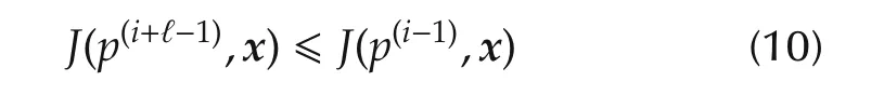
for some map J,then the solver S′that is derived from S by

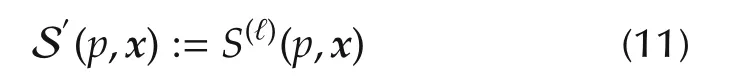
is monotonic in the sense of Definition 1 at the price of having a single iteration that takes ℓ-times longer than S,namely = ℓ·τS1.

The following assumption is needed for the updating algorithm that can be stated as follows:

Assumption 1The solver S is monotonic and the corresponding map J(see Definition 1)is bounded below by a strictly positive real J ,namely,

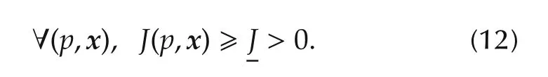
Note that the last condition(12)can always be satisfied by adding an appropriate positive constant to the original cost.

In order to recall the updating algorithm proposed in[7],the following notations are needed:

.J+k∶=J(p+(tk),(tk+1)):The cost function value for the initial hot start p+(tk)(before any iteration is performed)and based on the predicted state at the future updating instant tk+1=tk+q(tk)·τ.

.ˆJk+1∶=J(p(tk+1),(tk+1)):The cost function value for the delivered value p(tk+1)(after q(tk)iterations)and based on the predicted state at the future updating instant tk+1=tk+q(tk)·τ.

.Jk+1∶=J(p(tk+1),x(tk+1)):The effectively obtained cost function value for the delivered value p(tk+1)and for the true state x(tk+1)that is reached at instant tk+1=tk+q(tk)·τ.

Based on these definitions,it comes out that the decrease of the augmented cost function can be studied by analyzing the behavior of the ratio Jk+1/Jkwhich can be decomposed according to

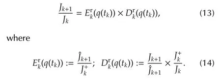
A deep analysis of the above terms shows that Erk(q)is linked to the current efficiency of the solver since it represents the ratio between the value of the augmented cost for the same predicted valueˆx(tk+1)of the state before and after q(tk)iterations are performed.The first ratio Jk+1/ˆJk+1in Drkis 1 if the model is perfect since it represents the ratio between two values of the augmented function for the same value p(tk+1)of the parameter but for two different valuesˆx(tk+1)and x(tk+1).Finally,the ratio J+k/Jkis linked to the quality of the hot start since it represents the predicted ratio between two values of the augmented function before and just after the horizon shift.

The algorithm proposed in[7]recalled hereafter updates the number of iterations q(tk+1)to be performed during the next updating period so that the contraction ratio:

is lower than 1 and if this is achievable,the updating rule tries to minimize the corresponding expected response time trof the dynamics which is linked to the ratio q/log(Krk+1(q)).

This leads to the following algorithm[7]:

Algorithm 1(Updating rule for q(tk+1))

1)Parameters qmax≤N,δ∈{1,...,qmax}.

2)Input data(available after step 3.2)page 95).

3)q=q(tk),p(0)=p+(tk),p(i)=S(i)(p(0),(tk+1)).

4)Jk,J+k,k+1,Jk+1.

5)Compute the following quantities:

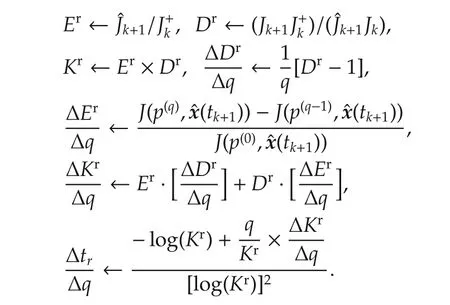
6)If Kr≥ 1,then

7)Output q(tk+1)←max{2,min{qmax,q−δ·sgnΓ}}.

Roughly speaking,this algorithm implements a step of size δ in the descent direction defined by the sign of the approximated gradient Γ.The step is projected into the admissible domain of q∈{2,...,qmax}.More details regarding this algorithm are available in[7].

Section 5 shows the efficiency of the proposed algorithm when applied to a given solver for the PLC-based implementation of MPC to the cryogenic refrigerator.Before this,the next section gives a simple argumentation that underlines a fundamental trade-off between the efficiency(per iteration)of a solver and the basic corresponding unbreakable computation time τS1.This is done in adaptation-free context in order to decouple the analysis.

2.3 Fundamental trade-off in the choice of solvers

Let us consider a solver S and the corresponding time τS1that is needed to perform the unbreakable amount of computations involved in a single iteration.Given a control updating period τu,the number of iterations that can be performed is equal toand the corresponding variation of the augmented cost function would be given by

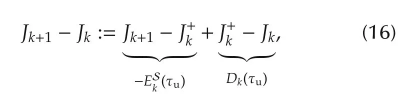
where here again,ESk(τu)and Dk(τu)are linked to the current efficiency of the solver(ESk)and the combined effect of model mismatch and the horizon shift effect on the cost function respectively.Both terms depend obviously on τu.Indeed ESk(τu)depends on τuthrough the number of iterations while Dk(τu)depends on τusince when τu=0 then Dkvanishes(no prediction error and no possible bad hot start).Note that ESkand Dkare absolute(non relative)versions of the relative maps Erkand Drkinvoked in Section 2.2 to introduce Algorithm1.Note also that unlike the efficiency indicator ESk(τu)which heavily depends on the solver,the Dk(τu)term is solver-independent.

Fig.1 shows typical evolutions of these terms for two different solvers S1(most efficient)and S2(less efficient).It can be seen that the iterations of S1are more efficientat the price of longer computation timeThe dots on the lower plot recall that the updating can be delivered only at quantized updating instants.

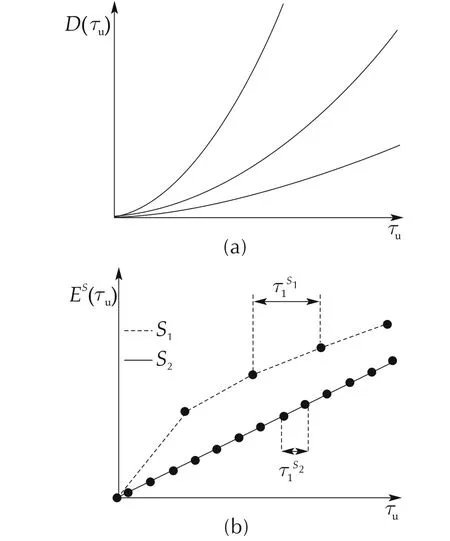
Fig.1 Possible evolutions of the Dk(τu)and ESk(τu)in realistic fast NMPC implementations.The lower figure shows the efficiency maps for two different solvers corresponding to two different computation times per iteration

Now based on(16),the decrease of Jkis conditioned by the inequality:

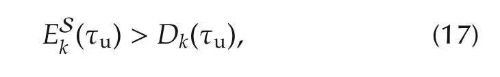
which expresses the need to have the ESkcurves above the Dkcurve for the adopted value of the updating period.

Fig.2 gives a qualitative illustration of the resulting fundamental trade-off:The upper plot shows situations where the use of the more efficient solver S1makes(17)impossible to satisfy regardless of the updating period being used.In such cases,the lower plot shows that less efficient solvers like S2together with appropriate short updating periods can satisfy the decreasing condition(17).The lower figure also shows that in this latter case,there may be several possible values of τu(several number of iterations)that may decrease the cost and an adaptive on-line monitoring algorithm like the one recalled in Section 2.2 may be appropriate to get closer to an optimal decrease.

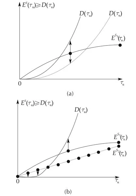
Fig.2(a)Use of the most efficient solver S1:depending on the context,there are possible configurations of D that make the decrease of the augmented cost impossible.(b)In such cases,the use of the less efficient solver S2enables to decrease the augmented cost thanks to shorter updating periods.

In the following sections, the two solvers that are used in the validation section are introduced.

3 Presentation of the algorithms

3.1 The qp OASES solver

The qpOASES[14]solver is a well know solver in the linear constrained MPC control community.It of-fers a very efficient implementation of the active-set strategy[13].If several quadratic programming(QP)problems must be solved with constant Hessian and constraint matrices,the qp OASES package offers the possibility of hot-starting from previous solution with a subroutine called qp OASES_sequence.In the sequel,the qp OASES_sequence subroutine will be used and will simply be recalled as qp OASES.

3.2 The ODE-based solver

In this section,an ODE-based solver that is used hereafter to implement the PLC-based constrained MPC is briefly presented.The real-time performance of this solver is also compared to that of qp OASES in the PLC constrained performance setting in order to illustrate Fact 1 mentioned above.

Consider the QP problem defined by

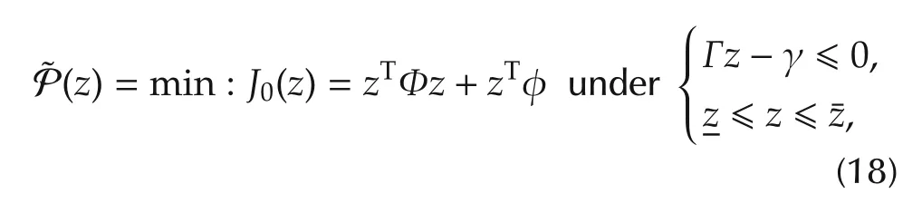
where z ∈ Rnzis the decision variable while Φ and φ are matrices of appropriate size.Γ ∈ Rnc×nzand γ ∈ Rncare the matrices that define the set of ncinequality constraints while z andare lower and upper bounds on the decision variables.

Based on the above formulation,the following augmented cost function can be defined:

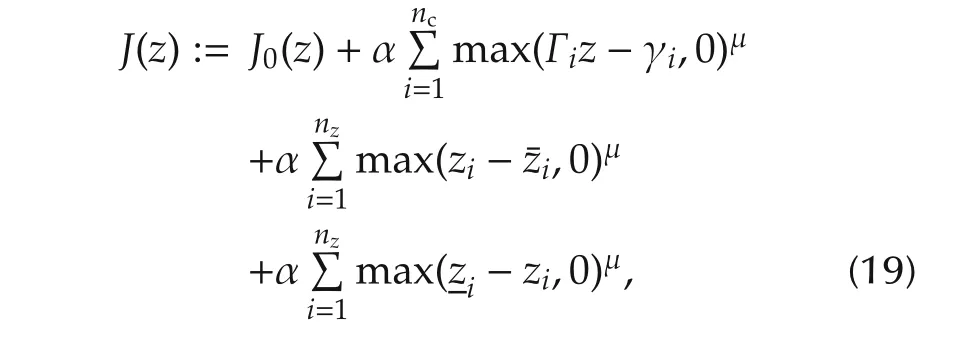
where Γi∈ R1×nzis the i th line of Γ while the typical value μ=2 is used hereafter.Based on this augmented cost,the following ordinary differential equation(ODE)can be used to define a trajectory in the decision variable space along which the augmented cost decreases:

Note however that this ODE is generally stiff because of the high values of αone needs to use in order to enforce the constraints fulfillment.That is the reason why the one-step backward-differentiation-formulae(TR-BDF2) described in [15] for stiff differential equations is used here.

Note also that after the computation of the TR-BDF2 step,all the decision variable that correspond to hard constraints(saturation on actuator for instance)are projected into the admissible box before a next iteration is computed.In addition to the integration scheme described in[15],the initial time step is defined by using the following expression:

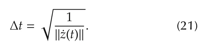
In the case of the quadratic problem described in Section 4.3,this method leads to fast convergence to the suboptimal solution z∗,being very close to the actual optimal solution of the original problem even with realtime constraints.The comparison between Sections 3.1 and 3.2 is given in Section 5.1.

Note also that this solver fully satisfies the decrease condition(9)since it moves along the descent trajectory defined by(20).Therefore,the adaptation mechanism of the control updating period can be applied.

4 Plant description

4.1 General presentation

Fig.3 shows an overview of the cryogenic plant of the CEA-INAC-SBT,Grenoble.This plant provides a nominal cooling capacity of 450W at 4.4K in the configuration in which this study have been done.It is dedicated to physical experiments (cryogenic component testing,turbulence and pulsed heat load studies,etc.).

The process flow diagram of the cryogenic plant is shown in Fig.4.One may notice the following main elements:

-Two volumetric screw compressors(NC∗)and a set of control valves(CV95∗),

-Several counterflow heat exchangers(NEF∗),a liquid nitrogen pre-cooler(NEF5),

-A cold turbine expander which extracts work from the circulating gas(Stt207),

-A so-called turbine valve(CV156),

-A Joule-Thomson expansion valve for helium liquefaction(CV155),

-A phase separator(NS1),connected to the loads(simulated here by the heating device referred as NCR22).

Note that the plant can be viewed as the interconnection of four elementary subsystems:the warm compression station(S4),the Nitrogen pre-cooler(S3),the Brayton cycle(S2)and the JT cycle(S1),delimited by dotted lines in Fig.4.While constrained MPC is used in this study,the cryogenic system is classically controlled by three independent control loops:

.The output temperature of the turbine expander is controlled with a PI controller working with the turbine valve CV156(%opening);

.the level of liquid helium in the tank is controller by a PI controller,working with the heating device NCR22(heating power);and

.the high and low pressures(in red and blue pipes,respectively)is controlled by an LQ controller,like the one described in[16].

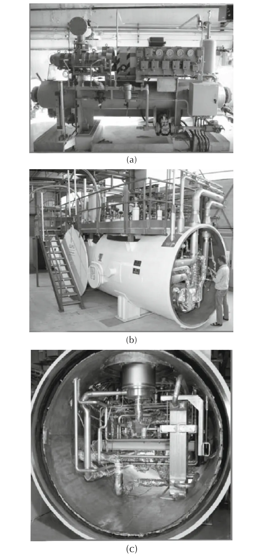
Fig.3 Views of the cryogenic plant of CEA-INAC-SBT,Grenoble.(a)The screw compressor of the warm compression station.(b)The cold box.(c)Internal detail of the cold box.

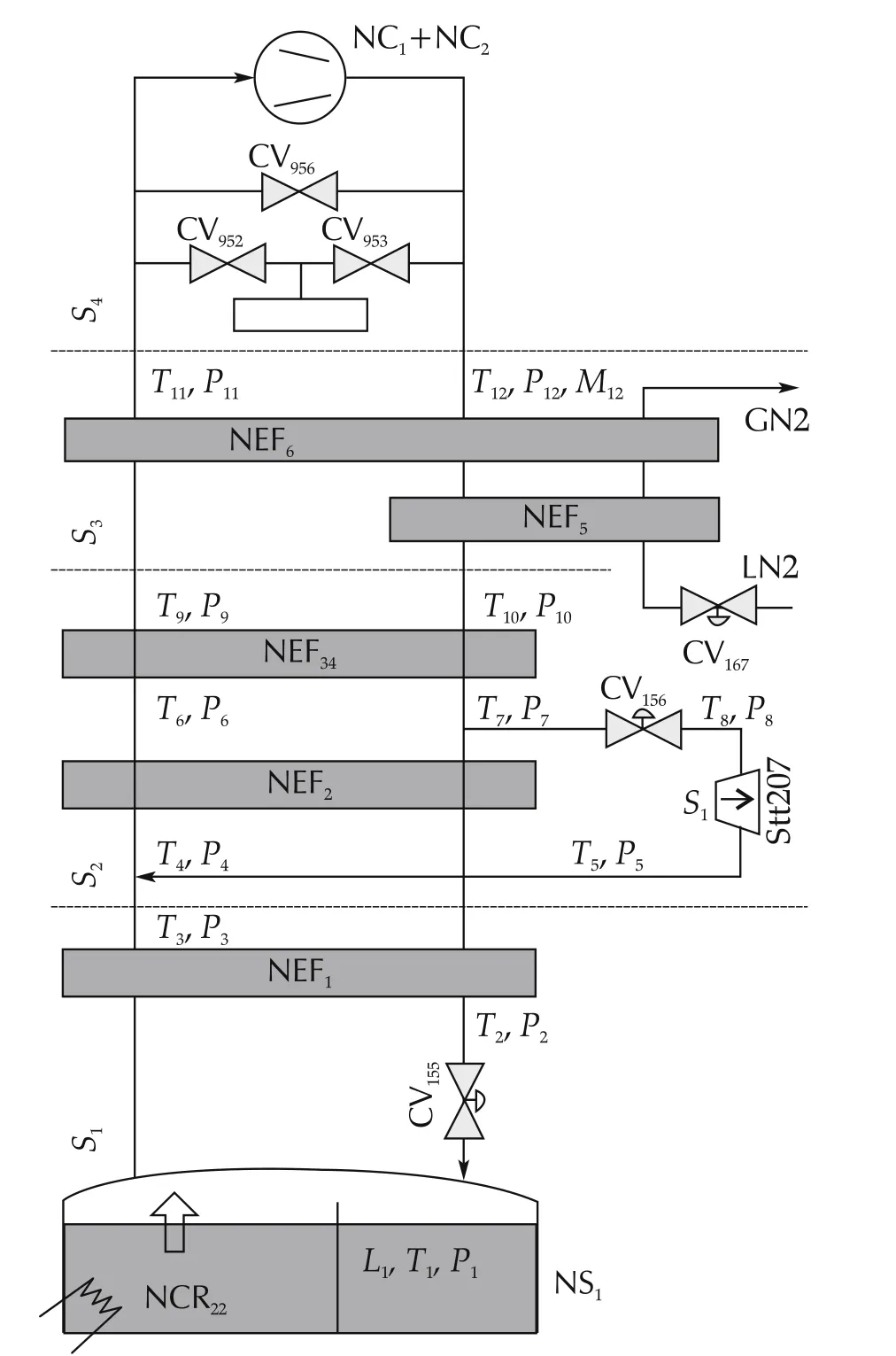
Fig.4 Functional overview of the 450W at 4.4K helium refrigerator available at CEA-INAC-SBT,Grenoble.The components named CV are controlled valves,used to control the system.The label Stt stands for the cryogenic turbine while NS is used for the phase separator.NC’s are helium compressors while NEF’s stand for heat exchangers.T’s and P’s stand for temperature and pressure sensors.S1is the turbine speed sensor while L1stands for the bath level sensor.

The valve CV155being used at a constant opening set by the user,depending on the application.In this study,attention has been focused on subsystems S1and S2,with are the coldest part of the refrigerator(from 80K to 4.4K).More informations about the plant can be found in[17].

4.2 Model derivation and properties

In order to derive the system model,several stu dies have been conducted[16–19].The Joule-Thompson cycle of this paper has been modelled in[19]while the Brayton cycle is presented in details in[16].It is worth mentioning that heat exchangers involve models with coupled partial differential equations(PDEs)that have been spatially discretized,leading to rather large state space.In this study,the two models has been merged to obtain a state space model that takes the following form:

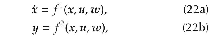
where f1is the function that express the derivative of the state x while f2is the function that express the measured output vector y.Both functions are continuously differentiable.State vector,input vector,and disturbance vector are expressed more precisely by

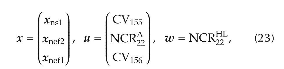
where xns1,xnef1and xnef2depict the state vector of individual components,described in[16,19].It has to be noted that NCR22is used both to control the plant and to disturb it.That is why it has been named NCRA22for the actuator part and NCRH22Lfor the heat load part.At the end,NCR22=NCRH22L+NCRA22.The vector of measured output is

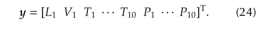
It has been shown in[19]that the nonlinear model expressed by(27)can be linearized around an operation point of interest defined by f1(x0,u0,w0)=0.The linearized model is then discretized using MATLAB function c2d(·)with sampling period τ=5s,leading to the following discrete LTI model:

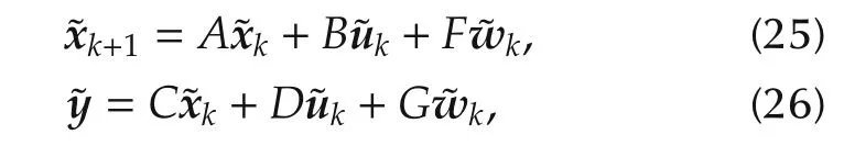
where variables with a tilde depict the deviation of the original variables around the operating point of interest:

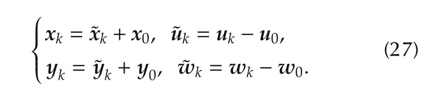
Note that the model defined by(26)stands for the prediction model(2)invoked in the general presentation of MPC(Section2.1).Following the same notation, the predicted output is denoted by yk+j=Y(j,xk,p,)while the true measured output is denoted by Yr(j,xk,p,).

4.3 Statement of the MPC-related optimisation problem

First of all,the following constraints have to be satisfied as far as possible:

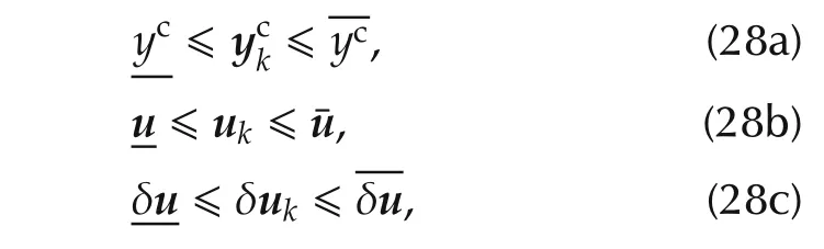
where δukstand for the increment uk−uk−1on the input vector.yckdenotes a subset of output components ykwhich is constrained.This subset is composed of the helium bath level L1and the turbine output temperature T5.Details regarding the variables involved in(28)are given in Table 1:

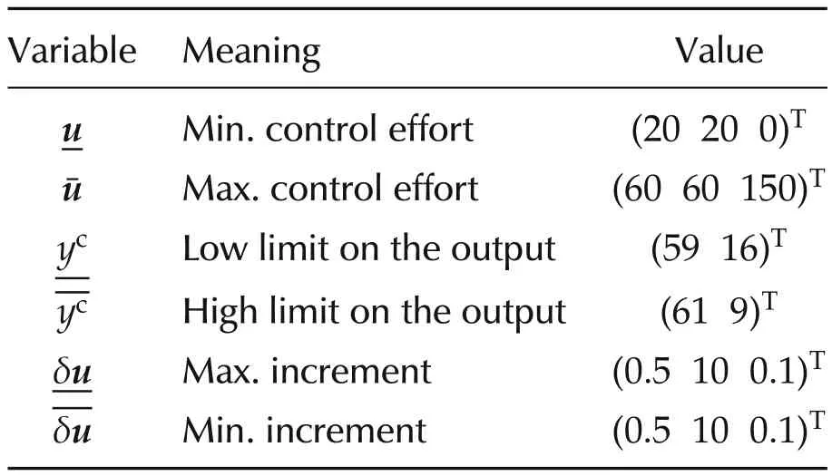
Table 1 The constraints bounds.

One of the specific features of output constraints is that they cannot be necessarily fully respected depending on the unpredictable thermal loads. That is why these constraints are systematically relaxed.This is introduced through the constraint violation variable υkthat is defined as follows:

while constraint violation prediction at sampling instant k+j is written:

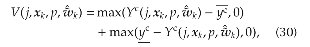
where Yc(j,xk,p,W)is used to define the constrained subset of Y(j,xk,p,W).

The sequence of control vectors u(i)(p)is then obtained by minimizing the cost function:

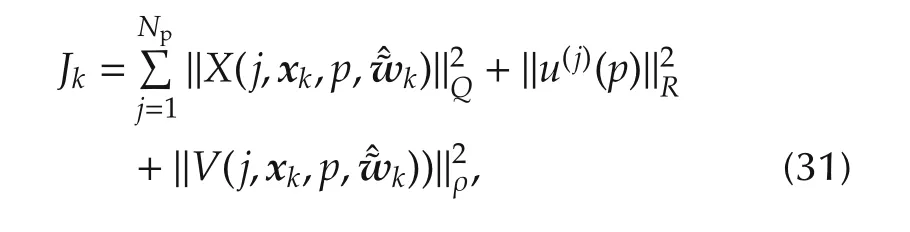
where Q and R are weighting matrices on the state and input vectors while ρ defines the constraint violation-related penalty.This cost function,together with the linear constrained and the linearized model(26)lead to a constrained QP problem which is of the form(18)in which the decision variable z is precisely the control profile parameter p.Note also that the affine term φ(see(18))does depend on the current value of the disturbance w=

By choosing a sampling period τ=5s,preliminary simulations showed that a prediction horizon of at least Np=100 is required.This leads to an optimization problem that involves 700 decision variables and a total number of 1000 constraints to be satisfied if trivial pwc parametrization is adopted.Such problem are beyond the computational capacity of the targeted industrial PLC(see the performance of our PLC in the Section 4.4).

To reduce the problem dimension,the control profile has been parametrized using classic piece-wise affine method that leaves as decision variables the values of the control inputs at 7 decisions instants1Decisions instants are chosen to be(1,2,4,8,16,50,50,100)..Moreover,the constraints satisfaction is checked only at 14 future instants2Constraints verifications instants are chosen to be(1,2,3,4,6,8,16,24,32,48,60,72,84,100)..This finally leads to an optimization problem involving49decision variables (note that there are7control inputs,namely 3 physical inputs and 4 virtual inputs virtual inputs representing the constraints violation),with56(outputs)plus 38 rate saturation constraints to be satisfied.

To ensure that this scheme is appropriate to control the plant,the problem closed-loop system is first simulated using the qpOASES solver.Time results are presented in Fig.5.

Fig.5(a)shows the thermal heat load that has been used in this simulation.Part(b)shows that the scheme is able to decrease the stage instantaneous cost defined as

Parts(c)and(d)of Fig.5 show that the constraints are violated within limited amplitude and duration.Part(e)shows the control effort.Part(f)shows the number of iterations of the qpOASES solver.It is worth mentioning that the number of iterations is important during heat load event.This has significant consequence on real-time feasibility of the qp OASES-based solution as it is examined in the sequel.

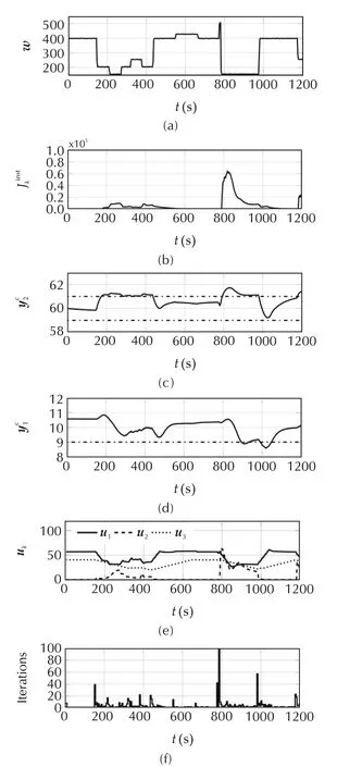
Fig.5 Simulated behavior of the system under qpOASES-based MPC control without limitation of the number of iterations.

4.4 Description of the PLC

This section focuses on the Programmable Logic Controller(PLC)available to implement the QP-based constrained MPC.It is a Schneider TSX P574634M shown in Fig.6.This PLC is fully dedicated to our application and it communicates optimisation results to another PLC that actually controls the plant.

Fig.6 Schneider PLC TSX P574634M.

According to the manufacturer,this PLC shows maximum computing capability of about 1.8M flops.In order to evaluate this claim,the Cholesky factorisation of increasing size matrices has been executed while monitored the computation times.Fig.7 shows the results and compares them to the performance of a nowadays DELL Latitude E6520 laptop with Intel I5-2520M CPU.This graph shows a slowing factor that lies around 4000.Note that the same graph shows the performance of the PLC in ms while the performance of the desk computer is shown in μs.

Note that the PLC is used with an external PCMCIA memory card of 2Mb,shared for both code and variables.This makes memory also a crucial issue.Indeed without reduced parametrization,the Hessian of the QP problem would have just fit the memory size of the PLC,since it represents a total memory occupation 4×7002=1.96Mb in single precision representation.

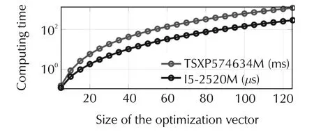
Fig.7 Cholesky factorisation time for two different CPUs.It can be noticed that the performance ratio between the PLC and the laptop is about 4000 for matrices sized 40 to 125.

Now since a single iteration of the qpOASES solver takes approximately 120μs,the same iteration would take 0.12×4000=0.48s when executed on the PLC.Therefore only 10 iterations of the qpOASES solver can be performed during the sampling period τ=5s.The scenario that has been shown in Fig.5 with no bound on the number of iterations has been simulated with the qpOASES “maxiter”option set to 10.The result is presented in Fig.8 on which the unlimited case has been also reported for easiness of comparison.

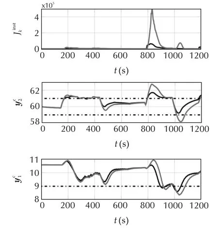
Fig.8 Simulated behaviour of the system under MPC control for both unconstrained(black lines)and constrained(grey lines)solving time.

Fig.8 shows that when the number of iterations of the hot-started qpOASES solver is limited to 10,the closed loop performance as well as the constraints fulfillment are drastically affected.This is precisely for this reason that the ODE-based solver explained in Section 3.2 has been developed since it corresponds to a less computation time per iteration and can therefore be potentially more suitable in presence of the limited performance available PLC following the discussion of Section 2.3.

5 Fast MPC-related investigation

5.1 Comparison of algorithms

The aim of the present section is to assess the first fact mentioned above,namely that it is sometimes better to use a less efficient per iteration solver(the ODE-based solver in our case)provided that it corresponds to less computation time per iteration.In our case,as far as the above described PLC is used,it is possible to perform 20 iterations of the ODE-based solver against only 10 iterations of the qpOASES solver.

Eight hours simulations have been done with the two solvers,with a variable computational capability(i.e.,a variable allowed number of iterations).Some relevant results are plotted,always as a function of the normalized computation capability=P/P0where P0is the computational capability of our device.

In order to support the comparison that can be difficult because of the presence of relaxed weighted constraints,the cost(31)to be minimized at each sampling period has been divided in two separated parts,in order to compare them separately.The first part represents the deviation cost:

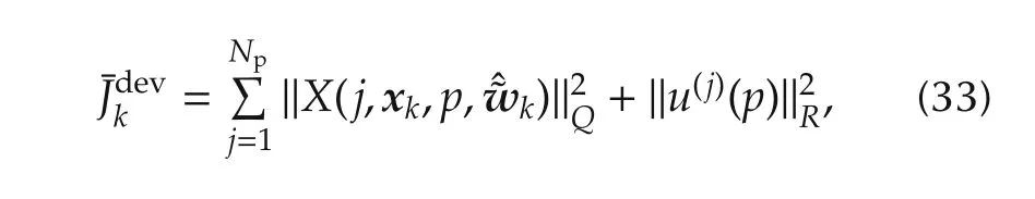
while the second part stands for the outputs constraints violation cost:

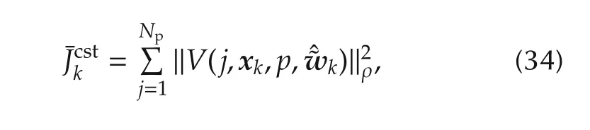
and then the sum of those two costs along the whole simulation is expressed:

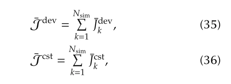
where Nsimis the number of problems solved during the simulation.

Then,constraints respect is presented in two different manners:

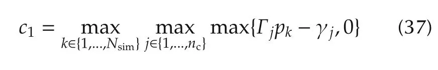
being the maximum predicted constraints violation during the simulation while

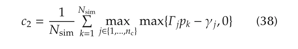
being the average predicted constraints violation during the simulation.

Finally,a closed-loop cost has been calculated according to

The quantities(35),(36),(35)+(36),(37),(38)and(39)are shown in Fig.9 against normalized computational performance¯P.It can be noticed that the suboptimal ODE-based solver is behaving better than qpOASES in the case of low performance computation devices,while the qpOASES solver becomes clearly better beyond some hardware performance indicator.

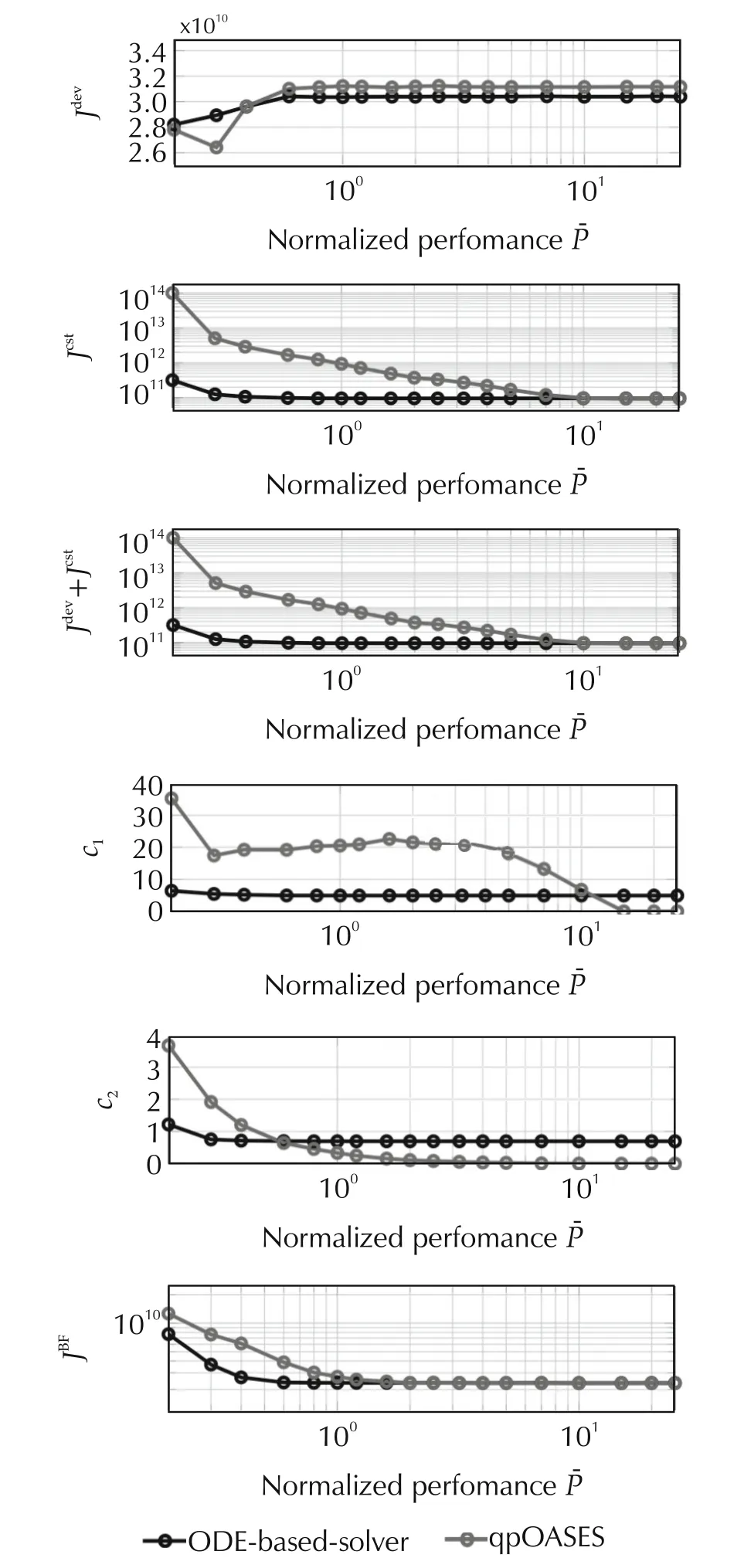
Fig.9 Performance indicators of the two solvers comparison vs the normalized computation power.The case¯P=1 corresponds to the PLC we dispose of and which is presented in Section 4.4.

The trajectories of the two closed-loop results are shown in Fig.10,comparing the two solvers for the nominal PLC performance P0against the result obtained with the qpOASES solver with limited number of iterations and with the 10 maximum number of iterations.

It comes clearly that the use of the less efficient(per iteration)solver with 20 iterations outperform the use of 10 iterations of the qpOASES solver.Moreover,the use of the ODE-based solver enables the nominal qpOASES(without limitation)performance to be recovered.

5.2 Control updating period monitoring

In the section,attention is focused on the ODE-based solver.First of all,simulations will be done for updating period from one to five(i.e.,a number of iterations from 4 to 20),and it will be shown that quadratic performances vary and there is an optimum to be found.Then the algorithm described in[7]and recalled in Section 2.2 will be implemented to show its efficiency on the cryogenic plant.

A six hour heat loads scenario presented by Fig.11 will be divided in six one hour parts,to be simulated.Cost(35)+(36)defined in the previous section will be plotted against the chosen updating period.The result is presented by Fig.12.It can be noted that the optimum updating period dynamically varies during the scenario.It illustrates the fact that the updating period should be monitored to enhance performance.

Fig.12 also plots the obtained performance by monitoring the updating period using the algorithm[7].It can be seen that it could lead to enhanced performances.

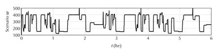
Fig.11 Six hours heat loads scenario.

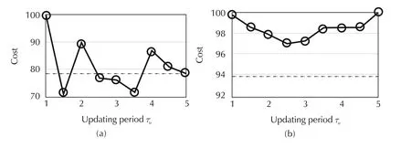
Fig.12 Normalized cost(35)+(36)against updating period(consequently the number of iterations)for six different scenarios named(a)to(f).Solid lines represent the cost while dotted lines depict the obtained costs with the algorithm described in[7]for δ=2.

6 Experimental results

The control scheme derived in Section 4.3 and the solver depicted in Section 3.2 has been implemented in the Schneider PLC described in Section4.4,in structured language.The objective of the section is triple.First,we want to show that the problem we derive in Section 4.3 is relevant regarding the control of a cryo-refrigerator submitted to transient heat loads.Then,we want to emphasize that the algorithm described in Section 3.2 is PLC compliant,even with polyhedral constraints.Finally,it is shown that monitoring the updating scheme is very useful in this particular cases.

6.1 Control result with real-time PLC implementation

The plant has been submitted to a two hours scenario(first two hours of Fig.11),starting from the equilibrium.The computation time per iteration is never longer than 250ms as expected.It allows the optimisation algorithm to iterate 4τu− 1 times(4 iterations per unit time with a safety term−1).For the first test,the control updating period τu=5s is first used.Fig.13 shows that the control scheme is able to stabilize the plant and to force a soft respect of the constraint,even if the plant is submitted to rather severe transient variable loads.

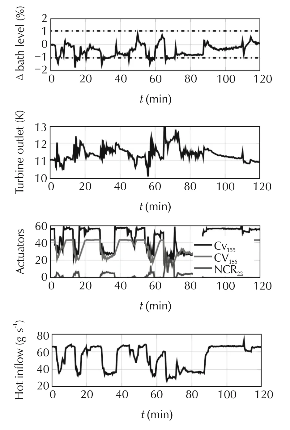
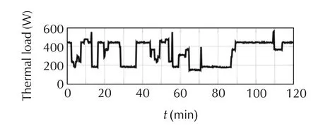
Fig.13 Two hours heat load scenario.This figure shows that the problem derived in Section 4.3 is relevant to control the plant.The Δ level represent the helium level L1 variation in the tank,Turbine stand for the output turbine temperature T5.The Inflow depict the high pressure flow M12coming in the cold-box.

6.2 Some leads on the updating scheme efficiency

The algorithm that adapts the control updating period on-line as been implemented on the PLC to show its efficiency.Fig 14 shows the difference between a constant updating period and a variable one.One can see that in the case of a serious change on the thermal load,the updating period is increasing to iterate more,while the algorithm is imposing a short updating period as soon as the problem is not changing much from an updating instant to another.

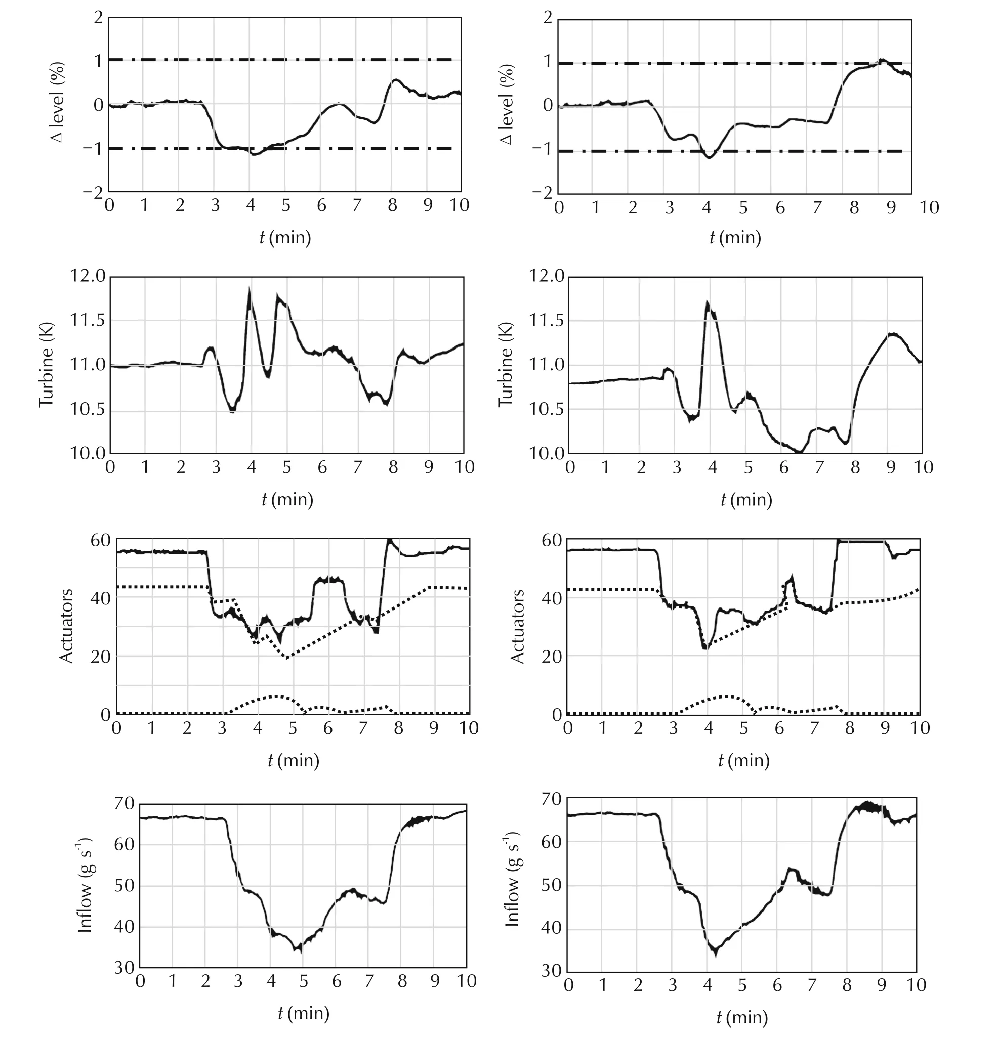
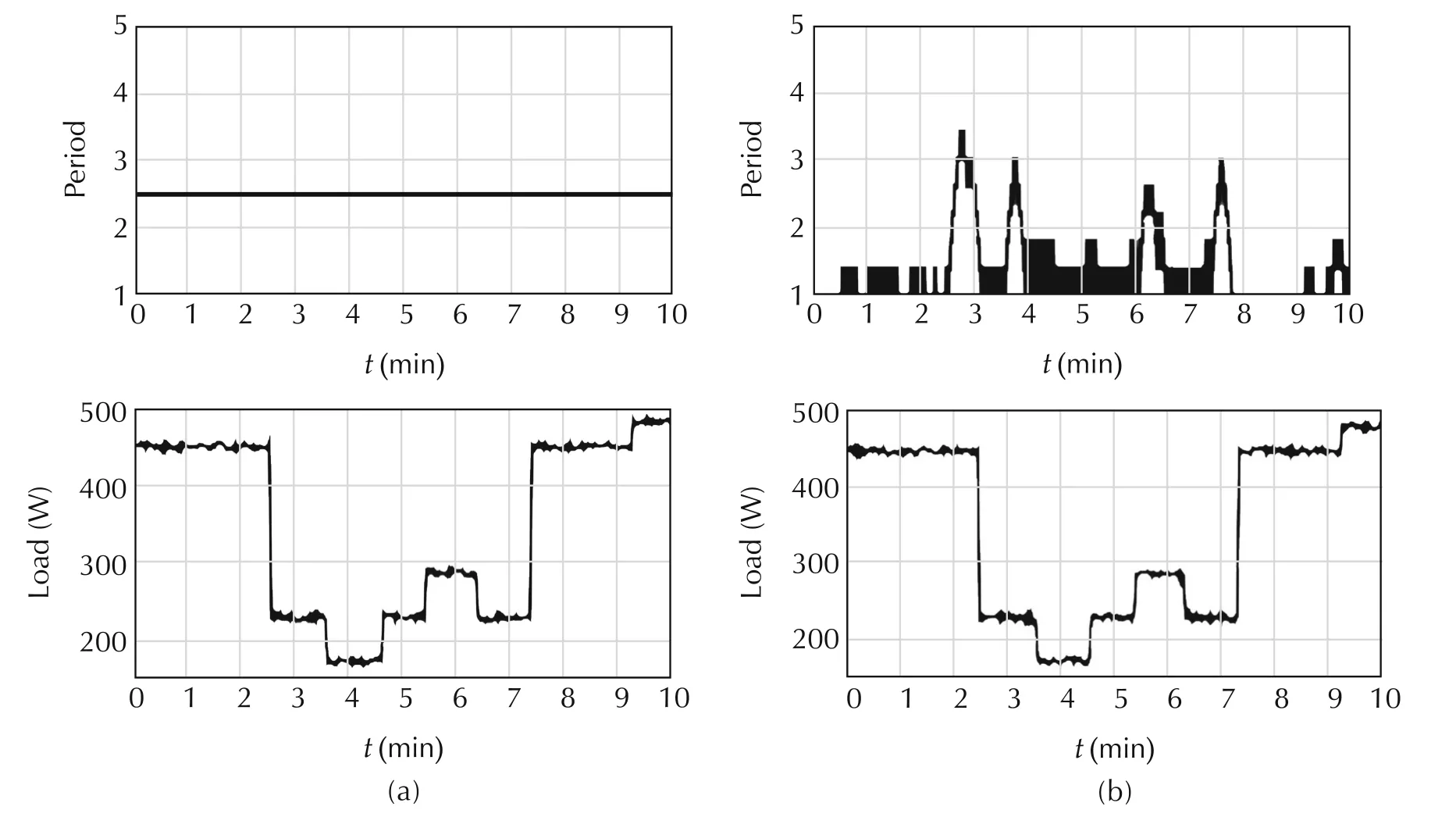
Fig.14 Result with both constant(2.5s)and real-time adaptation of the control updating period.It can be noticed that in the case of a heat load disturbance,the updating period is increasing(in order to make the number of iteration to also increase),since the hot-starting solution is far from the actual solution.Period represents the updating period τu.For actuators legend,please refer to Fig.4.

7 Conclusions and future work

In this paper,some aspects regarding the implementation of MPC in the case where the iterations performed by the solver should be stopped before a complete solution is obtained are discussed and illustrated through experimental real plant.

In particular,it has been shown that the choice of the appropriate solver depends on the available hardware.More precisely,in the presence of slow hardware,it might be advantageous to use less efficient(per iteration)solver in order to increase the updating rate.On the other hand,it has been shown that once the solver is chosen,monitoring the control updating period may improve the overall quality of the closed-loop or to reduce the computational burden for comparable performances.

This paper can be viewed as a concrete contribution to the today hot debate regarding on-line interrupted optimization-based MPC and its tight interaction with on-board computational devices.Although the best choice is context-dependent,this paper completes the series of conceptual contributions[6–9]through a concrete industrial application.

While the rather heuristic algorithm of[7]is used here,future works should take advantages of the more rigorous framework developed in[9]that explicitly incorporates certification results regarding the QP solver’s convergence in the adaptation scheme.A typical difficulty in such an attempt lies in the way some key parameters commonly used in expressing the certification results are to be estimated.

Acknowledgements

Authors would like to thank every co-worker from the SBT for their kind help to improve models and control strategy and for their time to correct and discuss this paper.Authors give special thanks to Michel Bon-Mardion,Lionel Monteiro,Fran¸cois Millet,Christine Hoa,Bernard Rousset and Jean-Marc Poncet from SBT for their explanation about the process and their participation on experimental campaigns.

[1]D.Q.Mayne,J.B.Rawlings,C.V.Rao,et al.Constrained model predictive control:Stability and optimality.Automatica,2000,36(6):789–814.

[2]M.Alamir.Stabilization of Nonlinear Systems Using Receding-Horizon Control Schemes:A Parameterized Approach for Fast Systems.Berlin:Springer,2006.

[3]M.Diehl,H.G.Bock,J.P.Schl¨oder.A real-time iteration scheme for nonlinear optimization in optimal feedback control.SIAM Journal on Control and Optimization,2005,43(5):1714–1736.

[4]V.M.Zavala,C.D.Laird,L.T.Biegler.Fast implementation and rigorous models:can both be accommodated in NMPC?International Journal of Robust and Nonlinear Control,2008,18(8):800–815.

[5]M. Diehl, R. Findeisen, F. Allgo wer, et al. Nominal stability of real time iteration scheme for nonlinear model predictive control.IEE Proceedings–Control Theory and Applications,2005,152(3):296–308.

[6]M. Alamir. A framework for monitoring control updating period in real-time NMPC schemes.Nonlinear Model Predictive Control.L.Magni,D.Raimondo,F.Allg¨ower(eds.).Berlin:Springer,2009:433–445.

[7]M.Alamir.Monitoring control updating period in fast gradient based NMPC.European Control Conference,Zurich:IEEE,2013:3621–3626.

[8]M. Alamir. Fast NMPC, a reality-steered paradigm: Key properties of fast NMPC algorithms.European Control Conference,Strasbourg:IEEE,2014:2472–2477.

[9]M.Alamir.From certification of algorithms to certified MPC:The missing links.IFAC-Papers Online,2015,48(23):65–72.

[10]A.Bomporad,Patrinos.Simple and certifiable quadratic programming algorithms for embedded linear model predictive control.IFAC Proceedings Volumes,2012,45(17):14–20.

[11]C. N. Jones, A. Domahidi, M. Morari, et al. Fast predictive control:Real-time computation and certification.IFAC Proceedings Volumes,2012,45(17):94–98.

[12]Y.Nesterov.A method of solving a convex programming problem with convergence rate O(1/k2).Soviet Mathematics Doklady,1983,27(2):372–376.

[13]H.Ferreau,H.G.Bock,M.Diehl.An online active set strategy to overcome the limitations of explicit MPC.International Journal of Robust and Nonlinear Control,2008,18(8):816–830.

[14]H.Ferreau,C.Kirches,A.Potschka,et al.qpOASES:A parametric active-set algorithm for quadratic programming.Mathematical Programming Computation,2014,6(4):327–363.

[15]R.E.Bank,W.M.Fichtner,W.Fichtner,etal.Transient simulation of silicon devices and circuits.IEEE Transactions on Electron Devices,1986,ED-32(10):1992–2007.

[16]F.Bonne,M.Alamir,P.Bonnay,et al.Model based multivariable controller for large scale compression stations.Design and experimental validation on the LHC 18kW cryorefrigerator.AIP Conference Proceedings,Anchorage:American Institute of Physics,2014:DOI 10.1063/1.4860899.

[17]F.Clavel,M.Alamir,P.Bonnay,et al.Multivariable control architecture for a cryogenic test facility under high pulsed loads:Model derivation,control design and experimental validation.Journal of Process Control,2011,21(7):1030–1039.

[18]F. Clavel. Mode´lisation et Controˆ le d’un Re´frige´rateur Cryog ´ enique.Application`alaStation800W`a4.5Kdu CEA Grenoble.Ph.D.thesis.Grenoble,France:University of Grenoble-Alpes,2011.

[19]F.Bonne,M.Alamir,P.Bonnay.Nonlinear observers of the thermal loads applied to the helium bath of a cryogenic Joule-Thompson cycle.Journal of Process Control,2014,24(3):73–80.

26 July 2016;revised 17 February 2017;accepted 17 February 2017

DOI10.1007/s11768-017-6109-y

†Corresponding author.

E-mail:mazen.alamir@grenoble-inp.fr.Tel.:+33-678115026;fax:+33-6476826388.

This work was supported by the French ANR Project CRYOGREEN.

©2017 South China University of Technology,Academy of Mathematics and Systems Science,CAS,and Springer-Verlag Berlin Heidelberg

Fran¸cois BONNEwas born in France in 1987.He received the M.Sc.in Control Systems from the University of Bordeaux,France,in 2011.Fran¸cois Bonne received his Ph.D.in 2014 from the Universite Grenoble Alpes,studying real-time model predictive control(MPC)applied to large scale cryo-refrigeration systems.He is now working with CEA(French atomic and alternative energy commission)to optimize the design and the operation of large scale cryogenic systems.E-mail:Francois.BONNE@cea.fr.

Mazen ALAMIRgraduated in Mechanics (Grenoble,1990)and Aeronautics(Toulouse,1992).He received his Ph.D.in Nonlinear Model Predictive Control in 1995.Since 1996,he has been a CNRS research associate in the Control Systems Department of the Gipsa-lab,Grenoble.His main research topics are model predictive control,receding horizon observers,nonlinear hybrid systems,signature-based diagnosis,optimal cancer treatment and industrial applications.He served as head of the“Nonlinear Systems and Complexity”research group in the Control Systems Department of the Gipsa-lab,Grenoble.Home page:http://www.mazenalamir.fr.E-mail:mazen.alamir@grenoble-inp.fr.

Patrick BONNAYwas born in France in 1971.He received the Graduate engineer of“conservatoire des arts et metiers”specialized in control systems in 2000.He’s been working for the CEA in the field of automation since 1994.He is currently the team leader of the Electronics and Control laboratory,and is responsible for the control systems of the cryogenic installations at the Low Temperature Service(SBT).During the past several years,he has been designing control system of cryogenics installations like the regulation of temperature of Laser Mega Joule target with a variation less than 1 Milli Kelvin and he has been actively involved in research projects which include model predictive control apply on cryogenics systems.Email:patrick.bonnay@cea.fr.