Modelling of Landslides:An SPH Approach

M.Pastor,T.Blanc,V.Drempetic,P.Dutto,M.Martín Stickleand A.Yagüe

Modelling of Landslides:An SPH Approach

M.Pastor1,T.Blanc1,V.Drempetic1,P.Dutto1,M.Martín Stickle1and A.Yagüe1

This paper presents a model(mathematical,rheological and numerical)for triggering and propagation of landslides presenting coupling between the solid skeleton and the pore fluid.The model consists of two sub models,a depth integrated model incorporating the propagation equations,and a 1D model describing pore pressure evolution.The depth integrated sub model is discretized using a set of SPH nodes,each one having an associated finite difference mesh for discretizing the pore pressure evolution.The model we propose differs from other depth integrated models with coupled pore pressures proposed in the past in the way pore pressures are described in the soil mass.Here,we will not restrict the analysis to an assumed shape function ful filling boundary conditions,but we will rather use a full approximation of pore pressures inside the landslide.

Landslide propagation, flowslides,depth integrated model,coupled vertical pore pressure,frictional fluid rheological model.

1 Introduction

Landslides cause severe economic damage and a large number of casualties every year around the world.Engineers and geologists need to understand and predict their properties,such as velocity,depth and run out distance.In addition to experience gained on similar cases,predictions require the application of mathematical,constitutive/rheological and numerical models.

In some cases,coupling between solid skeleton and fluids filling its voids is important,and properties such as run out and velocity depend on it.And because of pore pressures,friction seems to be smaller than that of the material.

Therefore,the mathematical model–the balance of mass and momentum equations–has to be able to reproduce this coupling and the evolution of pore pressures inside the landslide mass.

Depth integrated models present a good compromise between accuracy and computational cost,the 3D problem has been reduced to a 2D one.They have been extensively used since the pioneering work of Savage and Hutter(1989,1991),being worth mentioning the work of Iverson and Denlinger(2001),Hutter and Koch(1991),Naaim,Vial,and Coture(1997),Laigle and Coussot(1997),Pitman,Nichita,Patra,Bauer,Sheridan,and Bursik(2003),McDougall and Hungr(2004),Rodríguez Paz and Bonet(2005),Mangeney-Castelnau,Vilotte,Bristeau,Pertheme,Bouchout,Simeoni,and Yerneni(2003),Lajeunesse Mangeney-Castelnau,and Vilotte(2004),Pastor,Quecedo,Fernández Merodo,Herreros,González,and Mira(2002),D’Ambrosio,Iovine,Spataro,and Miyamoto(2007),Pastor,Haddad,Sorbino,Cuomo,and Drempetic(2009).

In most of the mentioned models,pore pressures are not taken into account.We can mention here the work of Hutchinson(Hutchinson 1986),who proposed a sliding consolidation model to predict run out of landslides,Iverson,and Denlinger(2001),Pastor,Quecedo,Fernández Merodo,Herreros,González,and Mira(2002),and Quecedo Quecedo,Pastor,Herreros,and Fernández Merodo(2003).

The effect of pore pressure has been described by Major and Iverson(1999),who provided experimental data describing the evolution of basal pore water pressure in debris flows,Iverson(2005).A more general approach–requiring more complex models-includes two fluids.Such models have been proposed by by Pitman and Le(2005)and Pudasaini(2012).

In the case of depth integrated models,all information concerning vertical pro files was condensed on a single variable describing basal pore pressure,and its evolution was modelled using simpli fied approaches.

The purpose of this paper is to propose a depth integrated model including vertical pro files of pore pressures.The latter are discretized using a simple finite differences explicit scheme,while the former model is discretized using a SPH model.In this way,problems such as making zero basal pore pressures-when the landslide crosses a terrain with very high permeability or a rack-can be modelled with more precision.Pore pressures are made zero at the base(imposing the boundary condition on the node located at the bottom),but are not zero at the whole mass of the soil.Indeed,when the avalanche leaves the zone,the boundary condition is changed again to zero flux.In models based on a single pore pressure variable it is not possible to take this effect into account.

Concerning pore pressure evolution,it is in fluenced by:

(i)Changes on landslide depth–because they generate changes in total vertical stresses.

(ii)Changes of soil dilatancy–the critical state line depends on the rate of deviatoric strain,as suggested independently by Pailha and Pouliquen(2009)and Pastor,Blanc,and Pastor(2009)

(iii)The basal surface over which the landslide propagates,which can be saturated,and generate a flow of water into the landslide mass resulting on a increase of pore pressure(or viceversa if the basal terrain is dilatant).

The paper is structured as follows:(i)First of all,in Section 2,we describe the mathematical model,which is based on Biot-Zienkiewicz model describing the coupling between solid skeleton and pore fluid.Equations for pore pressure evolution on 1D pro files are derived as a particular case,and a succinct description of the depth integrated model used is provided.

(ii)Section 3 is devoted to rheological modelling.We concentrate on diffuse failure mechanisms where the material is not necessarily of softening type.Then,we analyze additional sources of dilatancy–breaking of grains and rate of shear strain-and finish by describing a model for frictional fluids.

(iii)Section 4 deals with discretization,and presents the SPH model and the Finite Difference schemes associated to each SPH node.

(iv)Finally,Section 5 is devoted to present a number of examples and applications.

2 Mathematical model

2.1 Introduction

Geomaterials are mixtures of solids grains,liquids(water)and gases(air),presentingastronginteractionbetweentheirconstituents.Therefore,mathematicalmodels aiming to reproduce both triggering and propagation of landslides,have to take it into account.It is interesting to notice that two different paths have been followed to model the behavior of landslides.The former,based on geomechanics assumes the mixture is a solid,with small relative velocities of the fluid and gas phases relative to the solid skeleton,while the latter,considers the avalanching mass as a fluid with a particular rheological behavior.

In the case of the solid approach-geomechanical-we have to mention the pioneering work of Biot[Biot(1941);Biot(1955)]for linear elastic materials.This work was followed by further development at Swansea University,where Zienkiewicz and co-workers(Zienkiewicz and Shiomi 1984,Zienkiewicz,Chan,Pastor,Paul,and Shiomi(1990),Zienkiewicz,Xie,Schre fler,Ledesma,and Bicanic(1990),Zienkiewicz,Chan,Pastor,Shre fler,and Shiomi(2000)extended the theory to nonlinear materials and large deformation problems.It is also worth mentioning the work of Lewis and Schre fler(1998),Coussy(1995)and de Boer(2000).It can be concluded that the geotechnical community have incorporated coupled formulations to describe the behaviour of foundations and geostructures.Indeed,analyses of earth dams,slope failures and landslide triggering mechanisms have been carried out using such techniques during last decades.

In the case of the landslide propagation,coupled formulations have arrived later.We can mention here the work of Hutchinson[Hutchinson(1986)],who proposed a sliding consolidation model to predict run out of landslides,Iverson,and Denlinger(2001),Pastor,Quecedo,Fernández Merodo,Herreros,González,and Mira(2002),and Quecedo Quecedo,Pastor,Herreros,and Fernández Merodo(2003).

2.2 General model

The general model is based on the assumption that the mixture is composed of a solid phase and several fluid phases.The equations are:(i)balance of mass and(ii)balance of linear momentum for the constituents and the mixture,(iii)constitutive or rheological laws describing the material behaviour of all constituents,and(iv)kinematics relations linking velocities to rate of deformation tensors.The main problem with this approach is the computational cost,because of the number of unknowns and the dif ficulty of having to track all interfaces.The main advantage is its general character,as it can describe phenomena involving large relative displacements between solid and fluid phases.This model has been described by Pastor,Quecedo,Fernández Merodo,Herreros,González,and Mira(2002).

2.3 Biot-Zienkiewicz model

A first simpli fied model can be derived by assuming that the velocity of fluid phases relative to solid skeleton is small.In this case the equations can be cast in terms of the displacements or velocities of solid skeleton,the velocities of the pore water relative to the skeleton and the averaged pore pressure of the interstitial fluids.This model,proposedby ZienkiewiczandShiomi(1984)forthecaseof saturatedsoilsis referred to asu−pw−w.Its main variables are(i)the velocity of solid skeletonvs,(ii)the Darcy velocity of the pore water,wand the pore pressurepw.Under certain assumptions,which were analyzed for soil mechanics problems by Zienkiewicz and co-workers,it is possible to eliminate the Darcy velocity from the model.This is the most celebratedu−pwmodel of Zienkiewicz,which has been widely used in geomechanics being the base of many computer codes.The resulting model consists of the following equations:

•Balance of mass and momentum of pore water,which is obtained eliminating the Darcy’s velocity of the pore water:

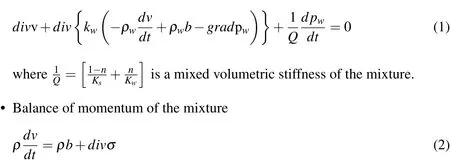
In above,v is the velocity of the soil skeleton,kwthe Darcy’s permeability,ρwand ρ the densities of the water and the mixture,b the body forces,pwthe pore pressure and σ the total stress tensor.

2.4 The propagation-consolidation approximation

So far we have described general models which can be applied to general problems.The analysis of landslides,due to their shape and geometrical properties allows some interesting simpli fications.First of all,we will arrive to“propagationconsolidation”models,where pore pressure dissipation takes place along the normal to the terrain surface,and next,we will describe depth integrated models,where the three dimensional problem is transformed into a two dimensional form.The propagation-consolidation model can be derived assuming that the velocity and pressure fields can be split into two components,i.e.,propagation and consolidation as v=v0+v and pw=pw0+pw1.

The equations of the propagation-consolidation model are:

where cvis the coef ficient of consolidation.

When applied to runout problems,we have to make two changes:

(i)As the soil column varies its height h,the pore pressure increases by an amount of

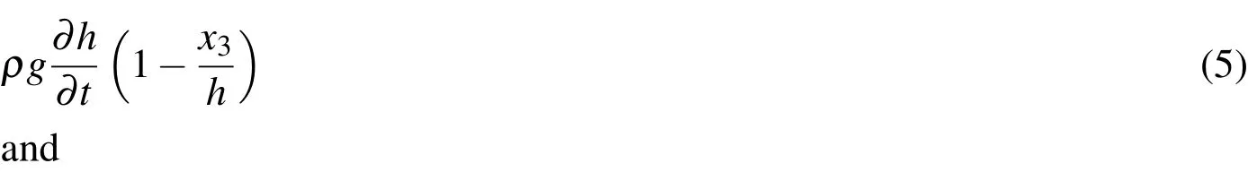
(ii)We have to account for large deformations in the X3 axis.

The final equation describing the vertical consolidation is:

It is interesting to note that two time scales exist in the equation,(i)a consolidation time,and another time related to the rate of variation of h.The solution depends on the ratio between both time scales.

2.5 Deth integrated equations

Many flow-like catastrophic landslides have average depths which are small in comparison with their length or width.In this case,it is possible to simplify the 3D propagation-consolidation model described above by integrating its equations along the vertical axis.The resulting 2D depth integrated model presents an excellent combination of accuracy and simplicity providing important information such as velocity of propagation,time to reach a particular place,depth of the flow at a certain location,etc.

Depth integrated models have been frequently used in the past to model flow-like landslides.ItisworthmentioningthepioneeringworkofSavageandHutter(1991);and the contributions of Laigle and Coussot(1997),Mc Dougall and Hungr(2005),and Pastor,Quecedo,Fernández Merodo,Herreros,González,and Mira(2002),and Quecedo,Pastor,Herreros,and Fernández Merodo(2003).We will use the reference system given in Figure 1 where we have depicted some magnitudes of interest which will be used in this section.

To derive a quasi lagrangian formulation of the depth integrated equations,we will first introduce a “quasi material derivative”as:

from where we obtain the “quasi lagrangian”form of the balance of mass,depth integrated equation as

Figure 1:Reference system and notation used in the analysis

whereeRis the erosion rate[L−1]andhis the flow depth The balance of momentum equation is

whereZis the height of the basal surface.

It is important to note that we have to include the effect of centripetal accelerations,which can be done in a simple manner by integrating along the vertical the balance of momentum equation,and assuming a constant vertical acceleration given byV2/R,whereVis the modulus of the averaged velocity andRthe main radius of curvature in the direction of the flow.

Concerning the consolidation equation,we will keep the full pro file along X3,therefore:

The model will be 2D(depth integrated),but with a 3D resolution of the pore pressure.

It is important to note that the results obtained above depend on the rheological model chosen,from which we will obtain the basal friction and the depth integrated stress tensor.

3 Modelling fluidized geomaterials behaviour

3.1 Introduction

Classical geomechanical constitutive equations are used most of the times to model the behaviour of solid soils,i.e.,before fluidization has occurred.This field has progressed very much in the last decades,from classical plasticity models to more advanced hypoplastic or generalized plasticity models.

There are excellent texts and state of art papers devoted to describe constitutive models and their use in geotechnical engineering.We can mention here the texts of Desai(1984),Cambou and Di Prisco(2000),Kolymbas(2000),Zienkiewicz,Chan,Pastor,Shre fler,and Shiomi(2000)among others,and the references provided therein.

On the other hand,models describing the behaviour of fluidized materials have been developed within the framework of rheology.

Rheological models have been developed since the work of Bingham(1922).In the case of cohesive fluids,exhibiting a yield stress,it is worth mentioning the contributions of Hohenemser and Prager(1932)and Oldroyd(1947)who generalized Bingham model for general stress conditions(see also Malvern(1969),Coussot(1994,1997,2005),Dent and Lang(1983),and Locat(1997).

If we assume that the fluid is isotropic,and we want to express the stress as a function of the rate of deformation tensor,it is possible to use the so called“representation theorems”.Following Malvern the stress tensor can be written as:

where p is a “thermodynamic”pressure,I the identity tensor,d the rate of deformation tensor,and Φkwith k=0.2 scalar functions of the invariants of d:

The invariants are de fined as:

In most of models it is assumed that the flow is incompressible,and therefore I1d=0.This is consistent with the decomposition into propagation and vertical consolidation described in the preceding Section,and also with the fact that soils fail at constant volume.However,the reader should be aware that this is just an assumption which has proven accurate only under certain assumptions.

In some cases,such as the Bingham model,the fluid is assumed to have cohesion,i.e.,a stress level below which no flow occurs.From a modelling point of view,this assumption introduces a computational problem,because the stresses are dif ficult to obtain,and special techniques have to be used.For an example,see Muravleva,Muravleva,Georgiu,and Mitsoulis(2010).

Therefore,theconsistentstudyofboththetriggeringandpropagationphasespresents the problem of having to use a constitutive model for the first part of the analysis and a rheological model for propagation.

As an alternative,Perzyna viscoplasticity provides a suitable framework within which both solid and fluid behaviour can be modelled.In a simple shear flow,a simple variant of Perzyna model can be written as:

where γ is a fluidization parameter and n a constant of the model which will be assumed to be 1.

And the Bingham fluid

The similitude of both formulations is clear.Of course,care has to be taken as a fluidized granular material can be compared to a fluid at early stages,but if the energy increases,it will become close to a granular gas.The approach of using viscoplastic models is therefore limited.

Moreover,models based on viscoplasticity do not present the ill-posedness nature exhibited by classical plasticity based models,where wave propagation velocities become imaginary in the softening regime[Sluys(1992)].

3.2 Perzyna models for soils

In the Perzyna model,the relation between the stress tensor and the strain tensor is given by

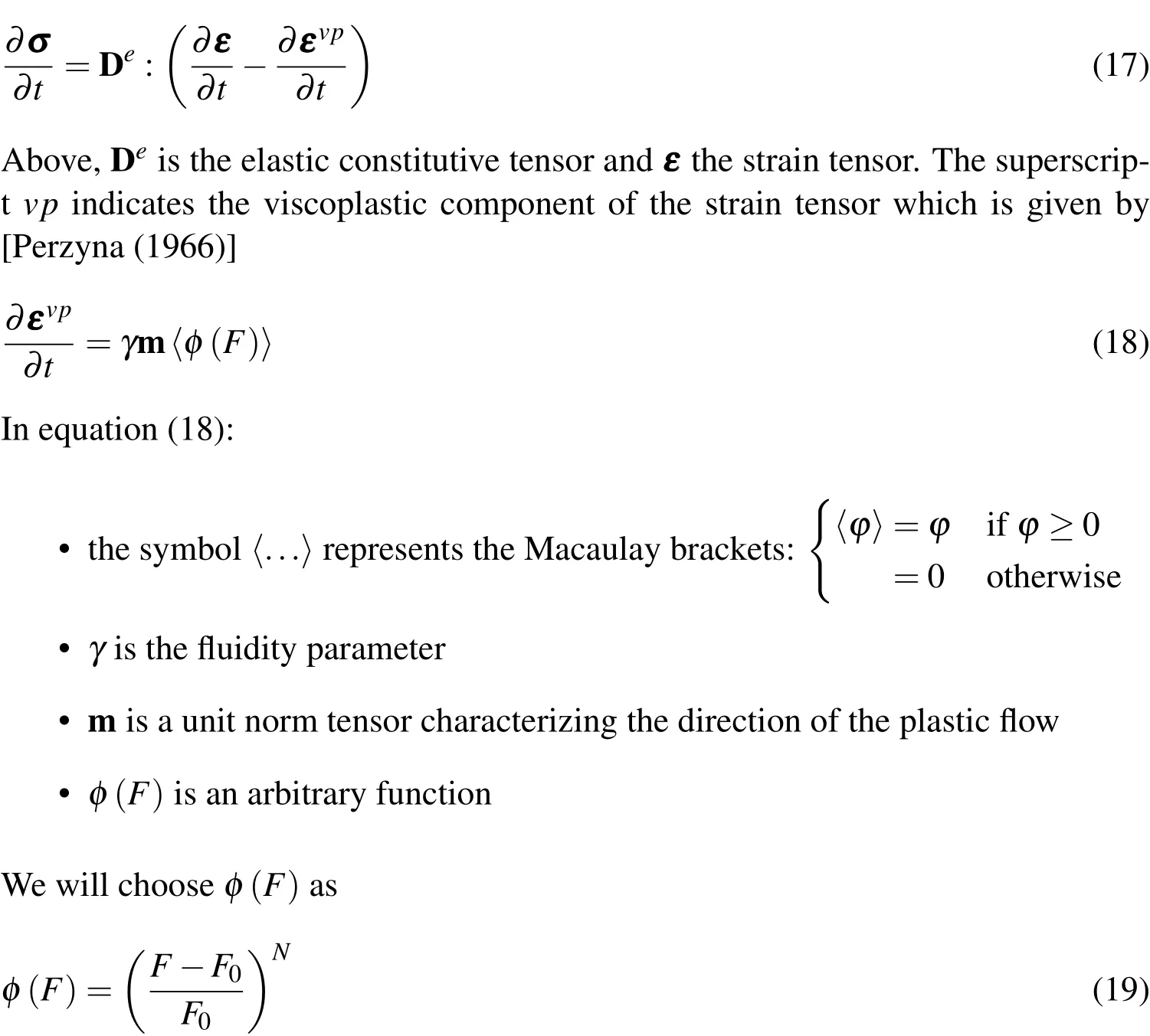
where N is a model parameter and F a function describing a convex surface in the stress space.The value F0characterizes the stress below which no viscoplastic flow occurs.

To complete the Perzyna model,the function F has to be de fined.In this paper,we will use two different functions F representing purely cohesive materials and clays:

a)The surface determined by the Von Mises yield criterion

b)The yield surface of the modi fied Cam-Clay model

a)The former yield criterion depends only on the second invariant of the deviatoric stress tensor,and is written as:

where q is related to Jby

2andY is a measure of the material cohesion.

We will choose F as

And the initial size of the yield surface will be given by

The size of the yield surface will vary according to a suitable hardening/softening law.Here we will assume that the size of the yield surface will be proportional to the increase of the equivalent deviatoric plastic strain,εvp

where H is the softening modulus.

We will also assume an associated flow rule,which means that the plastic potential surface g( σ )=0 coincides with the yield surface F( σ ,internalvariables)=0 and in consequence:

b)The yield surface of the modi fied Cam-Clay model has the form of an ellipsoid in the p−q plane and it is de fined as(Burland 1960):

where

p is the hydrostatic pressure

q is the deviatoric stress

M is the slope of the failure line in the p−q plane

Next,we will choose

The hardening/softening rule chosen is given by the relation between the size of the yield surface pcand the plastic volumetric strain,

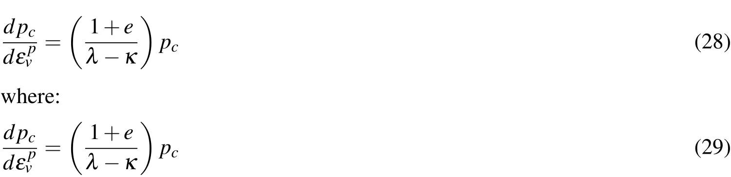
e is the void ratio of the material

λ is the slope of the ‘Normal Consolidation Line’

and κ is the slope of the line representing the unloading process in the p−q plane.

The flow rule will be associated,and therefore:

iii)The last governing equation is the kinetic relation between strain and velocities.This equation allows expressing the rate of deformation in terms of the gradient of velocity

where viis the velocity along the xiaxis.

The reader should be aware that the presented model is only valid for small deformations,and should be extended using a suitable objective form of the stress rate,such as that of Jaumann.However,this paper aims only to assess the capability of the

3.3 Depth integrated rheological models for fluidized soils

When obtaining the depth integrated equations described in the preceding Section,we have lost the flow structure along the vertical,which is needed to obtain both the basal friction and the depth integrated stress tensor.A possible solution which is widely used consist of assuming that the flow at a given point and time,with known depth and depth averaged velocities has the same vertical structure than a uniform,steady state flow.In the case of flow-like landslides this model is often referred to as the in finite landslide,as it is assumed to have constant depth and move at constant velocity along a constant slope.This in finite landslide model is used to obtain necessary items in our depth integrated model.We will present next some models frequently found in landslide propagation modelling.

3.3.1 Bingham fluid

In the case of Bingham fluids,there exists an additional dif ficulty,because it is not possible to obtain directly the shear stress on the bottom as a function of the averaged velocity.The expression relating the averaged velocity to the basal friction for the in finite landslide problem is,

where µ is the viscosity,τYthe yield stress,and τBthe shear stress on the bottom.

The pro files of velocities of Bingham fluids in in finite landslide models are characterized by the existence of a plug,or region where the stress is below the yield stress.No shear deformation appears,and the upper part of the flow moves rigidly,hence its name(Fig.2)

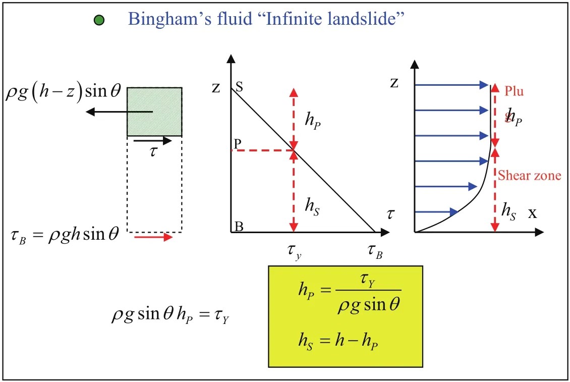
Figure 2:Velocity pro file of a Bingham fluid in an in finite landslide

3.3.2 Frictional fluid

One simple yet effective model is the frictional fluid,especially in the case where it is used within the framework of coupled behaviour between soil skeleton and pore fluid.Without further additional data it is not possible to obtain the velocity distribution.This is why depth integrated models using pure frictional models cannot include information concerning depth integrated stressesσ.Concerning the basal friction,it is usually approximated

where σvis the normal stress acting on the bottom.Sometimes,when there is a high mobility of granular particles and drag forces due to the contact with the air are important it is convenient to introduce the extra term.proposed by Voellmy’s[Voellmy(1955)],which includes the correction termwhere ξ is the Voellmy turbulence parameter.

In some cases,the fluidized soil flows over a basal surface made of a different material.If the friction angle between both materials δ is smaller than the friction angle of the fluidized soil,the basal shear stress is given by:

where the basal friction φbis

Thissimpli fiedmodelcanimplementtheeffectofporepressureatthebasalsurface.In this case,the basal shear stress will be:

We can see that the effect of the pore pressure is similar to decreasing the friction angle.

3.4 A viscoplastic based approach to rheological behaviour of fluidized soils

We will illustrate here the idea of describing fluidized soil rheology using Perzyna viscoplasticity.We have chosen the case of an in finite landslide,and analyzed it using the stress-velocity mixed finite element approach described in di Prisco,Pastor,and Pisanò (2011)and Pisanò and Pastor(2011).

In the case of the Von Mises model,the results are shown in Fig.3 below

We can notice the formation of a solid plug in the upper region of the flow,where the material has not yielded.

In the case of a Cam Clay model,the results are given in Fig.4.

We can see that velocity pro file differs from that of the purely cohesive soil,being close to a straight line.

4 Numerical models

4.1 Introduction

This section is devoted to present two of the models which we are using presently to model landslides.We have chosen the SPH(Smoothed particle hydrodynamics),a numerical technique allowing us the possibility to deal with large deformations avoiding expensive remeshing operations.

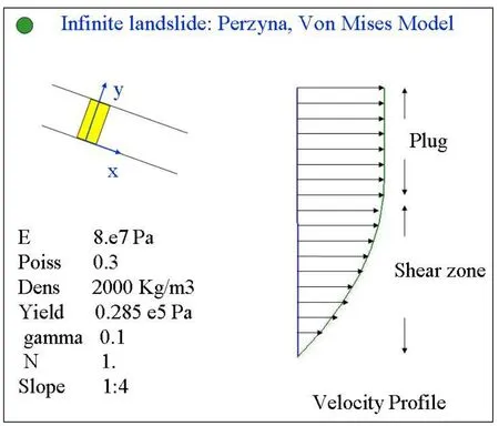
Figure 3:Velocity pro file obtained using a Perzyna Von Mises model

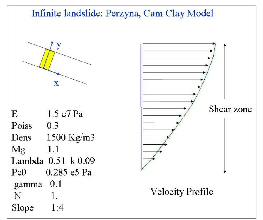
Figure 4:Velocity pro file in an in finite landslide obtained with a Cam Clay Perzyna model.

TheSmoothedParticleHydrodynamics(SPH)was firstappliedtomodelastrophysical problems[Gingold and Monaghan(1977);Lucy(1977)].From there,it was extended to classical hydrodynamics problems[Liu and Liu(2003)].Today SPH is used in many areas,among which it is worth mentioning magneto-hydrodynamics[Morris 1996)],multi-phase flows[Monaghan and Kocharyan(1995)],viscous flows[Takeda,Miyama,and Sekiya(1994)],quasi-incompressible flows[Monaghan(1994);Morris,Fox,and Zhu(1997)], flows through porous media[Zhu,Fox,and Morris(1997)],metal-forming[Bonet and Kulasegaram(2000)],impact problems[Randles and Libersky(1996)],elastic dynamics problems[Gray,Monaghan,and Swift(2001)],fast landslide propagation[McDougall(1998);M-cDougall and Hungr(2004);Pastor,Haddad,Sorbino,Cuomo,and Drempetic(2009)]and fluid structure interactions[Antoci,Gallati,and Sibilla(2007)].Recently and for the first time,SPH has been applied to soils problems involving soilwater interaction[Bui,Sako,and Fukagawa(2007)]and failure[Bui,Fukagawa,Sako,and Ohno(2008)].

Concerning the disadvantages and dif ficulties presented by the SPH method we can mention(i)The boundary de ficiency problems which can be solved by applying a normalization to the Smoothed Hydrodynamics method[Chen,Beraun,and Carney(1999)],and(ii)the tensile instability which appear in dynamics problems with material strength[Dyka,Brundsen,Schrott,and Ibsen(1995);Dyka and Ingel(1997);Swegle,Hicks,and Attaway(1995)].

We will present two SPH based models, first a Taylor SPH model where we formulate the mathematical model in terms of effective stress,pore pressure and velocity,and then,a depth integrated model which allows the approximation of consolidation pore pressure in 3D.

4.2 A Taylor SPH model for landslide analysis

The Taylor-SPH model has been presented by the authors in Blanc and Pastor(2010,2011,2012a,b).

The system of PDEs describing the behaviour of saturated soil are cast in terms of three fields:velocities,stresses and pore pressures.As in all mixed formulations,stability requires that the formulation satis fies the Babuska-Brezzi conditions.In our case,we ensure the stability of the stresses and velocities using a Taylor-Galerkin algorithm,whose stability has been shown by Codina(1998).

Coupled formulations have been shown to be unstable when displacements and pore pressures are discretized using the same approximation bases,unless special stabilization techniques are used.

Our SPH algorithm is based on the Fractional Step technique proposed by Chorin(1968),which was initially devised to use standard time-stepping schemes in incompressible fluid dynamics problems.

In the case of incompressible fluids,the Fractional Step algorithm consists of:

•Integrating the velocity in time without imposing the incompressibility con-

straint.We obtain an intermediate field v∗which is not divergency free

•Next,v∗is projected onto a divergence free space,which is done by solving

a pressure laplacian.

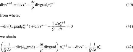
In the case of saturated geomaterials,the steps are the following:

•The intermediate velocity field v∗is obtained from:

In above,we have used what is called a full pressure projection,as we have not included the pressure gradient at time n in the first step.If we take the divergence of equation(39),we arrive at:

Therefore,the Fractional Step algorithm consists on:

–Obtaining the fractional velocity v∗using(37)

–Finally,vn+1is computed using(39).

Concerning discretization with SPH,the steps are the following:

(i)The first step is solved casting(37)together with the constitutive equation as a system of 1storder hyperbolic equations of the form

whereϕis the vector of unknowns,f is the flux tensor ands is the source vector.The source terms originate from body forces,Jaumann-Zaremba terms and viscoplastic rate of deformation tensor.This system of equations will be solved using an SPH version of the Runge-Kutta Taylor-Galerkin algorithm proposed by the authors(Blanc et al.(2011)]for solid and soil dynamics problems,where the equations are first discretized in space and then in time.

The arrangement of the SPH nodes is similar to that proposed by Randles and Libersky(2000).We will use an initial staggered node arrangement,which consist on a double set of SPH nodes(Fig.5).We call the nodes of the first set,the material SPH nodes,and the nodes of the second set,the auxiliary SPH nodes.It is interesting to note that auxiliary nodes play the same role than Gauss points in the finite element Taylor-Galerkin scheme.Thus each variable of the model is de fined at both material and auxiliary SPH nodes.

To approximate functions on the SPH nodes,only information coming from the SPH auxiliary nodes will be used and,vice versa,to approximate functions on the SPH auxiliary nodes,only information coming from the SPH nodes will be used.

Figure 5:SPH grid:material and auxiliary nodes

Values of the functionφand its spatial derivatives are approximated using the corrective SPH method which has been introduced to overcome the boundary de ficiency problem(Chen et al.1999).Using the corrective SPH method with the arrangement of SPH node presented above and the Taylor-Galerkin algorithm the SPH tensile instability is avoided(Blanc 2010).

(ii)The second step FS2 of the algorithm consists of computing the pore pressures at time tn+1solving a linear system of algebraic equations which coef ficients matrix arises from the discretization of the left hand side term of equation(42).The operator acting onis:

and involves discretization of the laplacian operator.We will use here the expression for the laplacian of scalar given by Schwaiger(2008):

where xIJ=xJ−xIand WIJ,αis the derivative of the kernel with respect to space coordinate α.

The discrete form of the pore pressure operator K can be represented by a n×n matrix;n being the number of SPH nodes.The right-hand side of the equation(45)is a vector of dimension n×1 which is easily obtained from the intermediate velocity v∗and the pore pressure at time n,pnw.The system K ·pn+1w=RHS is solved using a Preconditioned Jacobi Conjugate Gradient method.

Finally,in the third step,the projected velocity is obtained using equation(39)as:

which is easily discretized using the Corrected SPH method.

4.3 A Depth integrated SPH model for landslide runout analysis

We will introduce a set of nodeswith K=1...N and the nodal variables:

If the 2D area associated to node I is ΩI,we will introduce for convenience:

•a fictitious mass mImoving with this node mI=ΩIhI

•and,an averaged pressure term,given by

It is important to note that mIhas no physical meaning,as when node I moves,the material contained in a column of base ΩIhas entered it or will leave it as the column moves with an averaged velocity which is not the same for all particles in it.

Thereareseveralpossiblealternativesfortheequations,accordingtothediscretized form chosen for the differential operators results.We will show those obtained with the third symmetrised forms:

where we have introduced vIJ=vI−vJ.

Alternatively,the height can be obtained once the position of the nodes is known as:

The discretized balance of linear momentum equation is:

So far,we have discretized the equations of balance of mass and balance of momentum.The resulting equations are ODEs which can be integrated in time using a scheme such as Leap Frog or Runge Kutta(2ndor 4thorder).

Finally,we will have at each SPH node a 1D finite difference mesh which will be used to model pore pressure dissipation.The FD scheme is explicit because of both the simplicity and the speed of computation.

5 Examples and applications

5.1 Failure of a vertical slope under constant loading

We will present first an application of the Runge-Kutta Taylor-SPH algorithm described in Section 4.The case we have selected consists of the failure of a vertical cut under constant loading is studied.An analytical solution exists for the failure load of vertical slope and therefore it will give us an idea of the accuracy the Runge-Kutta Taylor-SPH algorithm.The vertical cut is modeled using a bi-dimensional approximation under plane strain conditions.The vertical cut is 10 meter high and 10 meters long.The footing is 5 meter width.Unlike the finite elements it is not required to model the footing(Figure 17).The boundary conditions in the area of the footing will represent the displacements due to the loading on the footing.

Figure 6:Sketch of the vertical cut and its discretization

The boundary conditions are(Figure 6):

The modulus of the velocityVtincreases constantly over time(Fig 7)

The material parameters are the elastic modulus:E=1·105Pa,the Poisson’s coef ficientν=0.35,the densityρ=2000 kg/m3.

The material is viscoplastic.The parameters of the Perzyna’s model and of the Von Mises yield criterion are the fluidity parameter:γ=2 s−1,the model parameter:

Figure 7:Boundary conditions of the vertical cut

N=1,the initial size of the yield surface Y0=200 Pa.In a first step the softening modulus is equal to 0:H=0 Pa in order to compare the failure load calculated by the Runge-Kutta Taylor-SPH algorithm to the analytical failure load.In a second step the softening modulus is H=−1·103Pa.

The analytical failure load,Panalytical,for a Von Mises material is given by:

In the Runge-Kutta Taylor-SPH algorithm,the failure load is calculated as:

Where:

NPare the eleven SPH nodes located under the footing

SPH nodes I and I+1 are consecutive SPH nodes of the boundary surface

σ22,Iis the vertical tension on SPH node I

xxxI,I+1is the vector formed by SPH nodes I and I+1

In order to compare the results obtained with the new Runge-Kutta Taylor-SPH algorithm to the analytical solution,the failure load is plotted in function of the displacement at base of the rigid footing(Figure 8).

In the perfect plastic case where no softening occurs,the load-displacement relationship of the SPH gives a response in accordance to the analytical solution of the problem.The curve rises linearly until 1000 N and then shows non-linear behavior,which correspond to plastic loading,until it reaches the collapse load.The analytical failure load is 1154 N and the estimated failure load given by our model is between 1171 N and 1267 N.In the case with softening the curve observed in the load-displacement relationship graph corresponds to the response imposed by the constitutive model.Indeed once irreversible viscoplastic deformations occur,the material starts to soften and then the failure load decreases.

Figure 8:Load-displacement curves:Analytical and computational solutions

The failure of the material is shown by the evolution of the deviatoric viscoplastic strains in the vertical cut(Figure 9).The viscoplastic deformations are accumulated in a sharp shear band clearly de fined.The shear band has an orientation of 45°which corresponds to the solution of the problem.In the first part of the calculation,thereareanydifferencebetweenthecaseofperfectviscoplasticityandthecasewith softening.However at the end of the calculation the shear band is better de fined in the case with softening.

The failure of the vertical cut is well illustrated when plotting the displacement contours on the deformed mesh(Figure 10).It appears two discontinuities where failure occurs:at the middle of the top border and at the middle of the right border.The right-upper triangle of the vertical cut is translated along the failure line represented by the shear band.The failure is sharper in the case with softening than in the perfect viscoplastic case.

This case study shows how accurate is the Runge-Kutta Taylor-SPH algorithm.The model is able to represent the sharp failure of a vertical cut under constant loading of a rigid footing.The viscoplastic deformations reach 73 percents in the case of perfect viscoplasticity and 60 percents in the case with softening.Thus the algorithm is useful to do a geotechnical analysis of a vertical cut in large deformation theory.

5.2 Breaking of a dam:frictional fluid

The firstexamplewewillconsiderhereisthatofthebreakingofadam.Wehaveassumed for the dam a height and a length of 10 m.Failure occurs instantaneously at time zero,and the material propagates along a horizontal plane.We have assumed an effective friction angle of 45°and a consolidation coef ficientCv=2.10−4m2s−1.

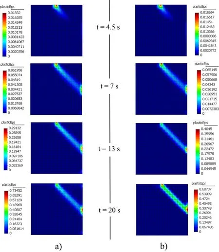
Figure 9:Evolution of the viscoplastic deformation in the vertical cut:a)perfect viscoplastic case;b)case with softening

The results are shown in figures 11 a to d,where we have plotted the pore pressure contours,which are given relative to those which cause liquefaction of the soil.It is important to see the differences with the dry soil case which is presented in Figs.12(a,b).

5.3 Aberfan flowslide of 1966

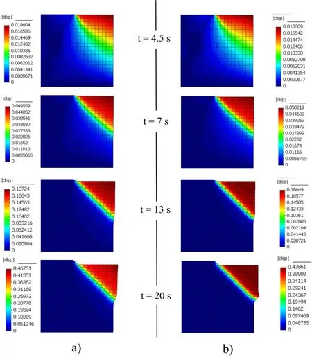
Figure 10:Displacement contours on the deformed mesh(Factor of deformation x2):a)perfect viscoplastic case;b)case with softening

One of the main dif ficulties when modeling Aberfan flowslide is the role of pore pressures.Coal debris were a material composed of solid, fluid and gas phases,with a strong interaction between them.However,models cast in terms of effective stresses,pore pressures,and velocities of all constituents have not been used so far,because of the problem of moving interfaces mentioned above.Depth integrated models can provide important information about runout,propagation paths and velocities,which is frequently suf ficient to design protection structures.The main shortcoming of depth integrated models comes from the fact that pore fluid and solid particles are modelled as a single phase material,with properties that do not change with time.This is why Aberfan flowslide has been modelled assuming a Bingham fluid rheological law for the debris.For instance,Jeyapalan et al.(1983)and Jin,Fread(1997)obtained results which fitted well the observations choosingτy=4794 Pa.,µ=958 Pa.s andρ=1760 kg/m3.Even if the results are good,it is possible to argue that waste coal was not fully saturated,and the material was frictional.Of course,the apparent angle of friction introduced above will be much smaller thanφ’,but vertical consolidation could have made it to change during the propagation phase.Hutchinson(1986)proposed a simple “sliding-consolidation”model in which it was clear that the combination of friction with basal pore pressures could provide accurate results of runout and velocities.

Figure 11:(a,b,c,d)Dam break:frictional saturated soil

This simpli fied method was used by the authors in[Pastor,Quecedo,Fernández

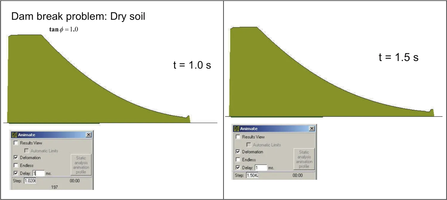
Figure 12:(a,b)Dam break:dry frictional soil

Merodo,Herreros,González,andMira(2002)].Itisassumedthatthereexistalayer of saturated soil of height hson the bottom of the flowing material[Hutchinson(1986)].The decrease in pore pressures is caused by vertical consolidation of this layer.Pore pressures on the top and bottom of this layer can be either estimated from the values of the vertical stresses or obtained directly from the results of finite element computations.

Assuming that the excess pore pressure evolves as

it is possible to obtain a closed form solution of the consolidation equation.In the case of

The coef ficientrucan be estimated as:

In above,we have used “pore pressures”instead of“pore water pressures”.The reason is that dry or partially saturated materials can collapse generating high air pressures on their pores,which will cause a similar effect.

The information provided in the literature do not provide enough data to perform a realistic analysis in two dimensions.Therefore,we have used a simple 1D model with the terrain pro files sketched in Fig.9,which are a better approximation than that of Jeyapalan et al.(1983).The main purpose of this example is to show that a depth integrated model using pore pressure dissipation can reproduce the basic patterns observed.

Therefore,we have used the vertical pro file given in Figure 13 below,where we can see the pro files both before and after the flowslide.

Figure 13:Vertical pro files of Aberfan tip before and after 1965 flowslides

Density of the mixtureρand friction angleφ’,have been taken as 1740 kg/m3and 36°respectively.we have chosencv=6.5.10−5m2/s.and assumed that a basal saturatedlayerof0.06timestheheightofthe flowslideatthebeginning.Initialpore pressure has been taken as 0.78 times the value corresponding to full liquefaction.The results obtained in the simulation are given in Figure 14 where sections of the free surface of the flowslide are given at times 0,6,10,15,20 and 30 s.In figure 15 we provide pore water pressure contours at time 2s.Please note that in order to improve readability,we have expanded the graphic representation of the saturated layer and it occupies the whole mass(This is possible because of the assumption that the saturated layer depth is proportional to that of the flowslide).

Figure 14:Vertical pro files showing Aberfan flowslide propagation

5.4 Effect of a terrain zone with very high permeability

One of the advantages of incorporating a set of finite difference meshes at each SPH node is the ability to improve the quality of the predictions in cases where basal pore pressures go to zero as a consequence of the landside crossing a terrain with very high permeability–or a rack.

The procedure to simulate this effect in the proposed model is based on changing the boundary condition associated to the finite difference nodes located at the contact with the terrain.

As a thought experiment,we will repeat the case presented in Section 5.3,including now such a zone.

We have selected the zone sketched in fig.16,where we have set the boundary condition of zero pore pressure at the bottom of all finite difference meshes associated to SPH nodes on it.

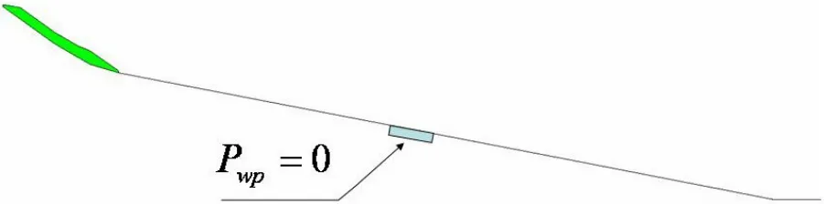
Figure 16:Location of the zero pore pressure zone

Figure 17 provides a comparison of the vertical pro files at different time stations.

Figure 15:Pore water contours at t=2 s.

Note that the depth has been ampli fied by a factor of 4.

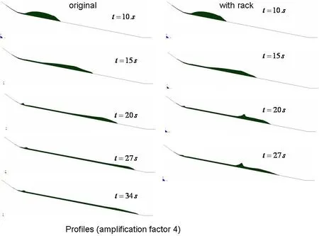
Figure 17:Vertical pro files at different times.Note the larger runout distance when no rack is present.

Concerning the distribution of pore pressure in the landslide, figures 18a and 18b provide the results obtained for times 17 and 20 s.The location of the rack is shown in fig.18b.

6 Conclusions

We have presented in this paper two alternative numerical models which can be used to describe triggering and propagation of landslides.

Concerning triggering,we have presented a coupled SPH model which avoids tensile instabilities inherent to classical SPH formulations.

Propagation is analyzed using a depth integrated SPH model which includes a vertical finite difference mesh providing higher accuracy of pore water dissipation.

Finally,and most important,we have shown how viscoplastic models of Perzyna type are able to reproduce the rheological behaviour of Bingham and frictional models.

Figure 18:(a)Pore water pressure distribution at time 17 s.(b)Pore water pressure distribution at time 20 s.

Acknowledgement:The authors gratefully acknowledge the economic support provided by the spanis Ministry MINECO(Projects GEODYN and GEOFLOW).The authors acknowledge the help of Dra.Mª.D.Elizalde for the help provided in the National Archives of UK(Kew)

Antoci,C.;Gallati,M.;Sibilla,S.(2007):Numerical simulation of fluid–structure interaction by SPH.Computers&Structures,vol.85,no.11,pp.879–890.

Bingham,E.C.(1922):Fluidity and Plasticity,McGraw-Hill,New York.

Biot,M.A.(1941):General theory of three-dimensional consolidation.J.Appl.Phys.,vol.12,pp.155–164.

Biot,M.A.(1955):Theory of elasticity and consolidation for a porous anisotropic solid.J.Appl.Phys.,vol.26,pp.182–185.

Blanc,T.;Pastor,M.(2012):A stabilized Fractional Step,Runge Kutta Taylor SPH algorithm for coupled problems in Geomechanics.Comput.Methods Appl.Mech.Engineering.,vol.221–222,1 May 2012,pp.41–53.

Blanc,T.;Pastor,M.(2011b):A stabilized Smoothed Particle Hydrodynamics,Taylor-Galerkin algorithm for soil dynamics problems.Int.J.Numer.Anal.Meth.Geomech.Published online in Wiley Online Library(wileyonlinelibrary.com).DOI:10.1002/nag.1082.

Blanc,T.;Pastor,M.(2011a):A stabilized Runge Kutta,Taylor Smoothed particle hydrodynamics algorithm for large deformation problems in dynamics.Int.J.Num.Meth.Engineering,vol.91,no.13,pp.1427–1458.

Bonet,J.;Kulasegaram,S.(2000):Correctionandstabilizationofsmoothparticle hydrodynamics methods with applications in metal forming simulations.International Journal for Numerical Methods in Engineering,pp.1189–1214.

Bui,H.H.;Sako,K.;Fukagawa,R.(2007):Numerical simulation of soil-water interaction using smoothed particle hydrodynamics(SPH)method.Journal of Terramechanics,pp.339–346.

Bui,H.H.;Fukagawa,R.;Sako,K.;Ohno,S.(2008):Lagrangian meshfree particles method(SPH)for large deformation and failure flows of geomaterial using elastic-plastic soil constitutive model.International Journal for Numerical and Analytical Methods in Geomechanics,pp.1537–1570.

Burland,J.B.(1965):Correspondence on “The yielding and dilatation of clay”.Géotechnique,vol.15,pp.211–214.

Cambou,B.;di Prisco,C.;(2000):Constitutive Modelling of Geomaterials.Hermes,Paris.

Chen,J.K.;Beraun,J.E.;Carney,T.C.(1999):A corrective smoothed particle method for boundary value problems in heat conduction.International Journal for Numerical Methods in Engineering,pp.231–252.

Chorin,A.J.(1968):Numerical solution of incompressible flow problems.Stud.Numer.Anal.,pp.64–71.

Codina,R.(1998):Comparison of some finite element methods for solving the diffusion-convection-reaction equation.Computer Methods in Applied Mechanics and Engineering,pp.185–210.

Coussot,P.(1994):Steady,laminar, flow of concentrated mud dispensions in open channel.J.Hydraul.Res.,vol.32,pp.535–559.

Coussot,P.(1997):Mud flow Rheology and Dynamics.Balkema,Rotterdam.

Coussot,P.(2005):Rheometry of pastes,suspensions and granular matter.John Wiley and Sons Inc.,Hoboken,New Jersey.

Coussy,O.(1995):Mechanics of Porous Media.John Wiley and Sons,Chichester.de Boer,R.(2000):Theory of porous media.Springer-Verlag,Berlin.

Dent,J.D.;Lang,T.E.(1983):A biviscous modi fied Bingham model of snow avalanche motion.Ann.Glaciol,vol.4,pp.42–46.

Desai,C.S.;Siriwardane,H.J.(1984):Constitutive laws for engineering materials with emphasis on geological materials.Prentice Hall.

diPrisco,C.;Pastor,M.;Pisanò,F.(2011):Shearwavepropagationalongin finite slopes:A theoretically based numerical study.Int.J.Numer.Anal.Meth.Geomech Article first published online:14 FEB DOI:10.1002/nag.1020.

D’Ambrosio,D.;Iovine,G.;Spataro,W.;Miyamoto,H.(2007):A macroscopic collisional model for debris- flows simulation.Environmental Modelling&Software,vol.22,no.10,pp.1417–1436.

Dyka,C.T.;Ingel,R.P.(1995):An approach for tension instability in smoothed particle hydrodynamics(SPH).Computers&Structures,pp.573–580.

Dyka,C.T.;Randles,P.W.;Ingel,R.P.(1997):Stress points for tension instability in SPH.International Journal for Numerical Methods in Engineering,pp.2325–2341.

Gingold,R.A.;Monaghan,J.J.(1977):Smoothed particle hydrodynamicstheory and application to non-spherical stars.Monthly Notices of the Royal Astronomical Society,pp.375–389.

Hohenemser,K.;Prager,W.(1932):Über die Ansätze der Mechanik der isotroperKontinua.Z.Angew.Math.Mech,vol.12,pp.216–226.

Hutchinson,J.N.(1986):A sliding-consolidation model for flow slides.Can.Geotech.J.,vol.23,pp.115–126.

Hutter,K.;Koch,T.(1991):Motion of a granular avalanche in an exponentially curved chute:experiments and theoretical predictions.Phil.Trans.R.Soc.London,vol.334,pp.93–138.

Iverson,R.M.(2005):Regulation of landslide motion by dilatancy and pore pressure feedback.J.Geophys.Res.,110,F02015,Doi:10.1029/2004JF000268.

Iverson,R.I.;Denlinger,R.P.(2001):Flow of variably fluidized granular masses across three dimensional terrain.1.Coulomb mixture theory.J.Geophys.Res.,vol.106,no.B1,pp.537–552.

Kolymbas,D.(2000):Introduction to Hypoplasticity.Balkema.

Laigle,D.;Coussot,P.(1997):Numerical modelling of mud flows.Journal of Hydraulic Engineering,ASCE,vol.123,no.7,pp.617–623.

Lajeunesse,E.;Mangeney-Castelnau,A.;Vilotte,J.P.(2004):Spreading of a granular mass on a horizontal plane.Physics of Fluids,vol.16,no.7,pp.2371–2381.

Lewis,R.L.;Schre fler,B.A.(1998):The Finite Element Method in the Static and Dynamic Deformation and Consolidation of Porous Media.J.Wiley and Sons.Liu,G.R.;Liu,M.B.(2003):Smoothed Particle Hydrodynamics a meshfree particle method.World Scienti fic Publishing,Singapore.

Locat,J.(1997):Normalized Rheological behaviour of fine muds and their flow properties in a pseudoplastic regime.In 1st International Conference on Debris-Flow Hazard Mitigation:Prediction and Assessment,Chen CL(ed),American Society of Civil Engineers,New-York,pp.260–269.

Lucy,L.B.(1977):Numerical Approach to Testing of Fission Hypothesis.Astronomical Journal,pp.1013–1024.

Major,J.J,;Iverson,R.M.(1999):Debris- flow deposition:Effects of pore- fluid pressure and friction concentrated at flow margins.GSA Bulletin,vol.111,no.10,pp.1424–1434.

Malvern,L.E.(1969):Introduction to the Mechanics of a continuous medium.Prentice-Hall.

Mangeney-Castelnau,A.;Vilotte,J.P.;Bristeau,M.O.;Perthame,B.;Bouchut,F.;Simeoni,C.;Yerneni,S.(2003):Numerical modeling of avalanches based on Saint Venant equations using a kinetic scheme.Journal of Geophysical Research,vol.108,no.B11,p.2527.

McDougall,S.(1998):A New continuum dynamic model for the analysis of extremely rapid landslide motion across complex 3D terrain.University of British Columbia.

McDougall,S.;Hungr,O.(2004):A model for the analysis of rapid landslide motion across three-dimensional terrain.Canadian Geotechnical Journal,vol.41,no.6,pp.1084–1097.

Monaghan,J.J.(1994):Simulating free surface flow with SPH.Journal of Computational Physics,pp.399–406.

Monaghan,J.J.;Kocharyan A.(1995):Sph Simulation of Multiphase Flow.Computer Physics Communications,pp.225–235.

Morris,J.P.(1996):Analysis of smoothed particle hydrodynamics with applications.Monash University.

Morris,J.P.;Fox,P.J.;Zhu,Y.(1997):Modeling low Reynolds number incompressible flows using SPH.Journal of Computational Physics,pp.214–226.

Muravleva,L.;Muravleva,E.;Georgiou,G.C.;Mitsoulis,E.(2010):Numerical simulations of cessation of a Bingham plastic with the augmented Lagran fian method.J.Non-Newtonian Fluid Mech.,vol.165,pp.544–550.

Naaim,M.;Vial,S.;Couture,R.(1997):St Venant Approach for Rock Avalanches Modelling in Multiple Scale Analyses and Coupled Physical Systems.Volume St-Venant Symposium Presse de l’Ecole Nationale des Ponts et Chausses.

Oldroyd,J.G.(1947):A rational formulation of the equations of plastic flow for a Bingham solid.Proc.Camb.Phil.Soc.,vol.43,pp.100–105.

Pailha,M.;Pouliquen O.(2009):A two-phase flow description of the initiation of underwater granular avalanches.Journal of Fluid Mechanics,vol.633,pp.115–113,doi:10.1017/S0022112009007460.

Pastor,M.;Blanc,T.;Pastor,M.J.(2009):A depth-integrated viscoplastic model for dilatant saturated cohesive-frictional fluidized mixtures:Application to fast catastrophic landslides.J.Non-Newtonian Fluid Mech.,vol.158,pp.142–153.

Pastor,M.;Quecedo,M.;Fernández Merodo,J.A.;Herreros,Mª.I.;González,E.;Mira,P.(2002):Modelling Tailing Dams and mine waste dumps failures.Geotechnique,vol.LII,no.8,pp.579–592.

Pastor,M.;Haddad,B.;Sorbino,G.;Cuomo,S.;Drempetic,V.(2009):A depth-integrated,coupledSPHmodelfor flow-likelandslidesandrelatedphenome-na.International Journal for Numerical and Analytical Methods in Geomechanics,pp.143–172.

Perzyna,P.(1966):Fundamental problems in viscoplasticity.Recent Advances in Applied Mechanics,vol.9,pp.243–377.

Pisanò,F.;Pastor,M.(2011):1D wave propagation in saturated viscous geomaterials:Improvement and validation of a fractional step Taylor-Galerkin finite element algorithm.Comput.Methods Appl.Mech.Engrg.,vol.200,pp.3341–3357.

Pitman,E.;Nichita,C.;Patra,A.;Bauer,A.;Sheridan,M.;Bursik,M.(2003):Computing granular avalanches and landslides.Phys.Fluids,vol.15,p.3638.

Pitman,E.B.;Le,L.(2005):A two- fluid model for avalanche and debris flows.Philosophical Transactions of the Royal Society A:Mathematical,Physical and Engineering Sciences,vol.363,no.1832,pp.1573–1601.

Pudasaini,S.P.(2012):A general two-phase debris flow model.Journal of Geophysical Research,vol.117,no.F3,F03010.

Quecedo,M.;Pastor,M.;Herreros,M.I.;Fernández Merodo,J.A.(2003):Numerical modelling of the propagation of fast landslides using the finite element method,Int.J.Numer.Meth.Engng,vol.59,pp.755–794,DOI:10.1002/nme.841.

Randles,P.W.;Libersky L.D.(2000):Normalized SPH with stress points,International Journal for Numerical Methods in Engineering,p.1445.

Rodíguez Paz,M.X.;Bonet,J.(2005):A corrected smooth particle hydrodynamics formulation of the shallow-water equations.Computers and Structures,vol.83,pp.1396–1410.

Savage,S.B.;Hutter,K.(1989):The motion of a finite mass of granular material down a rough incline.J.Fluid Mech.,vol.199,pp.177–215.

Savage,S.B.;Hutter,K.(1991):The dynamics of avalanches of granular materials from initiation to runout.Part I:Analysis.Acta Mechanica,vol.86,pp.201–223.

Schwaiger,H.F.(2008):An implicit corrected SPH formulation for thermal diffusion with linear free surface boundary conditions.International Journal for Numerical Methods in Engineering,pp.647–671.

Sluys,L.J.(1992):Wave propagation,localistation and dispersion in softening solids.Ph.D.Thesis,Delft University of Technology.

Swegle,J.W.;Hicks,D.L.;Attaway,S.W.(1995):Smoothed Particle Hydrodynamics Stability Analysis.Journal of Computational Physics,pp.123–134.

Takeda,H.;Miyama,S.M.;Sekiya,M.(1994):Numerical-Simulation of Viscous-Flow by Smoothed Particle Hydrodynamics.Progress of Theoretical Physics,pp.939–960.

Zhu,Y.;Fox,P.J.;Morris,J.F.(1997):Smoothed particle hydrodynamics model for flow through porous media.Computer Methods and Advances in Geomechanics,vol.2,pp.1041–1046.

Zienkiewicz,O.C.;Shiomi,T.(1984):Dynamic behaviour of saturated porous media:The generalised Biot formulation and its numerical solution.Int.J.Num.Anal.Meth.Geomech.,vol.8,pp.71–96.

Zienkiewicz,O.C.;Chan,A.H.C.;Pastor,M.;Paul,D.K.;Shiomi,T.(1990a):T.Static and dynamic behaviour of soils:a rational approach to quantitative solutions.I.Fully saturated problems.Proc.R.Soc.Lond.,vol.429,pp.285–309.

Zienkiewicz,O.C.;Xie,Y.M.;Schre fler,B.A.;Ledesma,A.;Bicanic,N.(1990b):Static and dynamic behaviour of soils:a rational approach to quantitative solutions.II.Semi-saturated problems.Proc.R.Soc.Lond.,vol.429,pp.311–321.

Zienkiewicz,O.C.;Chan,A.H.C.;Pastor,M.;Shre fler,B.A.;Shiomi,T.(2000),Computational Geomechanics,J.Wiley and Sons.

1ETS de Ingenieros de Caminos UPM Madrid Spain.