A Probabilistic Approach to Hazard Mapping Based on Computer Simulations.An Example for Lava Flows at Mount Etna

R.Rongo,D.D’Ambrosio,G.Iovine,F.Lucà,V.Lupiano,V.P.Boñgolan,W.Spataro

A Probabilistic Approach to Hazard Mapping Based on Computer Simulations.An Example for Lava Flows at Mount Etna

R.Rongo1,2,D.D’Ambrosio1,2,G.Iovine2,3,F.Lucà4,V.Lupiano5,V.P.Boñgolan6,W.Spataro1,2

Determining sectors that could be affected by lava flows in volcanic areas is essential for risk mitigation purposes.Traditionally,when adopting methods based on probabilistic numerical simulations,the hazard is assessed by analysing a huge set of simulations of hypothetical events,each characterized by a distinct probability of occurrence based on statistics of historical events.If lateral or eccentric eruptions are also taken into account,simulated lava flows usually start from the nodes of regular grids of potential vents,uniformly covering the study area.In this study,an alternative approach to evaluate flow-type hazard,based on a nonuniform grid of potential vents,is proposed.The method takes into account expected changes in the topographic context due to successive lava- flow bodies,and allows to obtain more detailed maps for the most exposed areas,besides signi ficantly reducing the computational efforts.The approach has been tested to evaluate lava- flow hazard at Mt Etna(Eastern Sicily,Southern Italy),and a preliminary analysis has been performed to investigate the behaviour of the adopted technique with respect to the number of performed sets of simulations to better understanding its predictive capability.

Probabilistic approach,non-uniform grid,hazard mapping,lateral/eccentric eruption,lava flow,Mt.Etna.

1 Introduction

Lava flows frequently threaten people and properties worldwide.About 10%of the world’s population lives next to volcanoes that are expected to show renewed activity,more than half a billion people in four big cities being exposed to volcanic risk[Peterson(1986);Chester,Degg,Duncan,and Guest(2001);Tilling,Norton,and Ridgway(2006)].

Volcanoesaregenerallycharacterizedbyinherentlyunpredictablebehaviours[Melnik and Sparks(1999)].Nevertheless,such systems are constrained by physical laws,showing systematic trends of evolution and periodic behaviour.Accordingly,the forecasting of volcanic activity represents a challenging research topic.

The hazard induced by lava flows is commonly evaluated by means of empirical geological approaches[e.g.Frazzetta and Romano(1978)],empirical–statistical evaluations[e.g.Behncke,Neri,and Nagay(2005)],or statistical-probabilistic analysis of past events[e.g.Sheridan and Macías(1995)].Available approaches can be distinguished into deterministic and probabilistic[Gómez-Fernández(2000)],in some cases also combined together[cf.Wadge,Young,and McKendrick(1994)].Deterministic methods generally involve the mapping of density of potential sources(lateral or eccentric vents),and attempt to identify the exposed areas by considering the potential propagation of the flows from such sources: flows are assumed to originate at given sites,and the threatened sectors are mapped by geomorphologic assessment.On the other hand,in probabilistic methods,physical models are commonly employed:a set of possible sources is assumed,and numerical simulations are performed for each of them,according to pre fixed types of events that characterize the study area.

Several authors recently employed massive,computer-based numerical simulation to evaluate lava- flows hazard at Mt.Etna[e.g.D’Ambrosio,Rongo,Spataro,Avolio,and Lupiano(2006);Crisci,Iovine,Di Gregorio,and Lupiano(2008);Iovine(2008);Crisci,Avolio,Behncke,D’Ambrosio,Di Gregorio,Lupiano,Neri,Rongo,and Spataro(2010);Tarquini and Favalli(2010);Rongo,Avolio,Behncke,D’Ambrosio,Di Gregorio,Lupiano,Neri,Spataro,and Crisci(2011);Cappello,Vicari,and Del Negro(2011);Del Negro,Cappello,Neri,Bilotta,Hérault,and Ganci(2013);D’Ambrosio,Filippone,Marocco,Rongo,and Spataro(2013a)],in Southern Italy.Indeed,a similar approach was also used to evaluate debris flows hazard in Campania[Iovine(2008);Avolio,Di Gregorio,Lupiano,and Mazzanti(2013);Lucà,Avolio,D’Ambrosio,Crisci,Lupiano,Robustelli,and Rongo(2013);Lucà,D’Ambrosio,Robustelli,Rongo,and Spataro(2014)]:a regular lattice of potential sources,uniformly covering the study area,is applied,and an exhaustive phase of numerical simulations of the overall potential flows is performed for each source,adoptedtypesofsimulationsbeingrepresentativeoftheconsideredphysical system.Once the computational phase is done(this is generally a time consuming step),a probability of occurrence is assigned to each simulation.By overlapping all the simulated flows and summing their probabilities,a probabilistic hazard map can be obtained.

Such type of classic approach has both advantages and shortcomings:among the pros,any change of values of the parameters affecting the probabilities of the simulations does not imply the need of re-executing the whole set of simulations,thus allowing the prompt updating of the hazard maps.In other words,the simulation phase is independent from the assignment of probabilities and from the evaluation of the hazard.In addition,a highly detailed map can be obtained for the entire study area,depending,among others,on the detail of the grid of potential sources covering the study area.Nevertheless,the method requires a massive computational effort,based on an elevated number of independent simulations(these latter may be distributed among different processing units aiming at reducing the overall computational time).Moreover,it does not consider the modi fications of the volcano in time,due to emplacement of new lava flows on the slopes.

An alternative method for evaluating flow-type hazard,based on a non-uniform grid of potential vents as in D’Ambrosio,Iovine,Lupiano,Rongo,Spataro,and Boñgolan(2013b),has been developed,aiming at i)further improving the details of the results for the most exposed areas,ii)accounting for possible modi fications of the topographic conditions in time,and iii)reducing the computational efforts.Non-uniform distributions allow for finer details of simulation in the most threatened sectors.Such type of grid was already used in speci fic areas of interest of computational domains:for instance,Blottner(1975)attempted to capture the turbulence in a boundary layer by this approach.While non-uniform grids frequently appear in adaptive methods,they may also be used in a static environment,as in Boñgolan-Walsh,Duan,Fischer,Ozgokmen,and Iliescu(2007),where the grid was purposely set finer at the inlet of the flow,and coarser downstream,to better capture the dynamics of evolving gravity currents.

In the present study,this alternative method was applied to evaluate the lava- flow hazard at Mt.Etna(Eastern Sicily,Southern Italy),the largest subaerial active volcano in Europe.Its flanks were repeatedly affected by lava flows from flank eruptions in historical times[Romano and Sturiale(1982)].In its eastern portion,a high spatial density of fractures,effusive fissures and pyroclastic cones is to be found[Mazzarini and Armienti(2001);Behncke,Neri,and Nagay(2005)],mainly along a SSE-trending fracture system which crosses the study area between the villages of Nicolosi and Trecastagni[Corazzato and Tibaldi(2006)].Moreover,deep-seated gravitational sliding towards the Jonian Sea,associated with larger-scale volcano-tectonic dynamics,affects the whole south-eastern flank of the volcano[Borgia,Ferrari,and Pasquarè(1992)],thus contributing to the volcanic evolution.First examples of maps outlining sectors of Mt.Etna mostly exposed to volcanic risk were realized by Frazzetta and Romano(1978),followed by Guest and Murray(1979),Duncan,Chester,and Guest(1981),Forgione,Luongo,and Romano(1989),and Behncke,Neri,and Nagay(2005).In the past few decades,signi ficant urban development has occurred mainly on the southern flank of the volcano,thus notably modifying the exposure of the elements at risk.

In the following,the new alternative method is described,and an application on distributed-memory machines to evaluate the lava- flow hazard at Mt Etna is presented.The computational speci fications of the numerical simulation phase are described,and 4 different probabilistic hazard maps,related to temporal frames ranging from 1 to 100 years,are presented.The behaviour of the adopted approach with respect to the number of performed sets of simulations is also preliminarily investigated.

2 Method and application to Mt.Etna

The alternative method for lava- flow hazard evaluation,here described,relies on numerical simulations of hypothetical flows that may originate in the study area,based on a non-uniform grid of potential vents,and on their subsequent elaboration in a GIS environment.After fixing a reference temporal frame,a set of maps(snapshots)is obtained:each derives from a computational run,by sequentially simulating a number of potential flows from a subset of probabilistically activated vents.For each snapshot,the number of simulations to be performed depends both on the observed frequencies of historical eruptions and on the extent of the considered temporal frame.The type of each simulation,expressed in terms of intensity(e.g.erupted volume over duration),also depends on historical observed frequencies.Thanks to the sequential strategy of execution within a given run,the simulated flows modify the topography(due to solidi fication),and may then affect the path of subsequent flows.At the end of each computational run,the cells of the snapshot are assigned the value 1 in case they are affected by one or more lava flows,or 0 if they are not affected.To obtain a statistically consistent result for the considered temporal frames,a proper number of snapshots must be computed and averaged,thus providing for reliable probabilistic hazard maps(in the following,PHMs).

In this study,lava flows were simulated by using Sciara-fv2[Spataro,Avolio,Lupiano,Trun fio,Rongo,and D’Ambrosio(2010)],a Cellular Automata(CA)model[cf.von Neumann(1966);Saravakos and Sirakoulis(2014);Was and Lubas(2014);Blecic,Cecchini,Trun fio,and Verigos(2014)].CA are parallel computa-tional models widely used for simulating the dynamics of systems whose evolution can be described in terms of local interactions among their constituent parts.They are dynamical systems,discrete in space and time.The space is subdivided into cells of uniform size and the overall dynamics of the system emerges as the result of the simultaneous application,at discrete time steps,of atransition functionto each cell,which takes as input the state of the cells belonging to theneighbourhood.Since such systems are made of independent cells,CA can be easily implemented on parallel computers[e.g.Setoodeh,Adams,Gürdal,and Watson 2006;D’Ambrosio and Spataro(2007)].

More in detail,Sciara-fv2 belongs to the family of Complex CA,also known as Macroscopic or Multi-component CA[cf.Di Gregorio and Serra(1999);Avolio,Di Gregorio,Spataro,and Trun fio(2012)],successfully applied to several types of complex,natural phenomena,such as lava and debris flows and forest fires[e.g.,Crisci,Di Gregorio,Rongo,and Spataro(2005);Di Gregorio,Filippone,S-pataro,and Trun fio(2013);Trun fio,D’Ambrosio,Rongo Spataro,and Di Gregorio(2011);D’Ambrosio,Filippone,Rongo,Spataro,and Trun fio(2012)].In a Multicomponent CA,the set of states is decomposed intosubstates,whilst thetransition functionis split intoelementary processes.Moreover,external in fluencesand physical/empiricalparameterscan be considered to account for global properties of the phenomenon to be simulated.In Sciara-fv2,substates are used to describe physical properties(e.g.lava thickness and temperature),while elementary processes allow to model substates changes in time(e.g.variations of thickness and temperature,and solidi fication of lava flows).Lava feeding at the vents is simulated by means of an external in fluence,as it would not be easily described in terms of local interactions.Eventually,a set of parameters accounts for physical properties,such as lava temperatures at the vents and at solidi fication,lava density and specific heat.For each step of computation,the model simulates the lava flows among the cells,and accounts for lava solidi fication depending on temperature changes.As a consequence,topographic modi fications are obtained step by step,until the flows stop at the end of a given simulation,and complete solidi fication occurs.Sciara-fv2 was successfully employed in previous applications to large study areas[e.g.,Crisci,Avolio,Behncke,D’Ambrosio,Di Gregorio,Lupiano,Neri,Rongo,and Spataro(2010);Rongo,Avolio,Behncke,D’Ambrosio,Di Gregorio,Lupiano,Neri,Spataro,and Crisci(2011);D’Ambrosio,Filippone,Marocco,Rongo,and Spataro(2013a)],where a signi ficant number of simulations had to be performed.More details on the model can be found in the above cited references,and in S-pataro,Avolio,Lupiano,Trun fio,Rongo,and D’Ambrosio(2010),and in Oliverio,Spataro,D’Ambrosio,Rongo,Spingola,and Trun fio(2011).

In this paper,the application of the method to Mt.Etna allowed to obtain lava-flow hazard maps for the following temporal frames:Δt1=1,Δt2=25,Δt3=50 and Δt4=100 years.The number of simulations performed in a computational run depends on the selected temporal frame,on one side,and on assumptions on the behaviour of the physical system under consideration(i.e.the volcano),on the other.For instance,if the system can be assumed in steady state,the mean number,s,of eruptions expected within a given temporal frame can be simply obtained by multiplying the duration of the temporal frame,Δt,by the mean number of historical events per year,m:

Furthermore,aiming at guaranteeing statistical variability,the actual number of simulations tobe simulated inthe i-th run,si,canbe selected byassuming a Poisson distribution of probability,havings as mean.To de fine the number of events to be simulated in each run,the mean number of lava flows per year at Mt Etna was first evaluated by analysing the historical behaviour of the volcano.In Tab.1,duration and volume of historical lava- flow events in the past 400 years are listed[Behncke,Neri,and Nagay(2005)].Among them,cases with extreme intensities(e.g.duration longer than 240 days,volumes greater than 160×106m3)were neglected,being considered quite improbable.Accordingly,a total of 52 types of eruptions were considered,with a mean number of expected events per year=52/400=0.13.By assuming a steady behaviour of the volcano,the mean numberss(Δtj)of expected events for the remaining framesof interest Δtj,j=2,...,4,were computed,again by applying equation 1.Obtained values are listed in Tab.2.

The above averages were taken as averages for randomly generating the number of simulations to be performed in each run,according to a Poisson distribution of probabilities,as shown in Fig.1.Speci fically,a random number c∈[0,1]was generated,by means of a roulette-like procedure,to entering the cumulative probability:the related abscissa(rounded at the next integer)indicated the numberof simulations to be performed in the i-th run of the j-th temporal frame.

In this study,the Probability Density Function(PDF)proposed by Lupiano(2011)was considered(with minor changes,see below),and a non-uniform grid of potential vents was adopted:the distribution of the sources is a function of the PDF,with greater densities in sectors characterized by higher probabilities of source opening(Fig.2).The adopted PDF takes into account the historical distribution of lateral and eccentric vents,and the distribution of the main faults/weakness structures of the volcano.With respect to the original proposal,the distance of the vents from the summit was not considered,to avoid overweighting of probabilities in sectors already marked by high structural weaknesses.

Table 1:Types of historical eruptions at Mt.Etna[Behncke,Neri,and Nagay(2005)].For each combination of volume(V,in 106m3)and duration(D,in days),the number of lateral eruptions recorded since 1600 A.D.are listed.Bold values mark the cases actually considered in this study

Table 2:For each temporal framethe mean number of expected eventsand the total number(rounded)of expected simulations over a total of r=240 computational runs are listed.The numbers of performed simulations,obtained by considering the Poisson distributions with meanare also reported for each temporal frame.The total number of both expected and performed simulations are also listed(in Italics)at bottom.

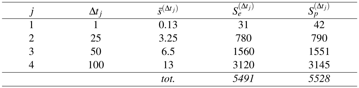
Table 2:For each temporal framethe mean number of expected eventsand the total number(rounded)of expected simulations over a total of r=240 computational runs are listed.The numbers of performed simulations,obtained by considering the Poisson distributions with meanare also reported for each temporal frame.The total number of both expected and performed simulations are also listed(in Italics)at bottom.

j Δtjs(Δtj)S(Δtj)eS(Δtj)p 1 1 0.13 31 42 2 25 3.25 780 790 3 50 6.5 1560 1551 4 100 13 3120 3145 tot. 5491 5528

Figure 1:a)Adopted Poisson cumulated distributions of probability(∑Pi),and b)distributions of probability(Pi)to determine the number of simulations to be performed for the considered temporal frames.

More in detail,the probability of opening of new vents was de fined based on the eruptive history and on geological characteristics of Mt.Etna(e.g.faults,dykes,eruptive fissures,lateralandeccentricvents)[cf.Ferrari,Garduno,andNeri(1991);Acocella and Neri(2003);Behncke,Neri,and Nagay(2005)].The PDF therefore de fines the likelihood that a vent will open in the considered sector,assuming that the probability increases in the vicinity of weakness structures as possible routes of ascent of magma.The likelihood is assessed according to the spatial density of eruptive fissures in the cell neighbourhood,this latter de fined by thekernel density estimation function[Silverman(1986)].In particular,theGauss kernel[Connor and Hill(1995)]was adopted,thanks to its characteristics of symmetry and ability to describe the typical mechanisms of mass transfer and temperature in volcanic systems.Theoptimal distancewas evaluated by comparing the observed distances amongthe eruptivefractures withthe theoretical curves(expected distribution),and applying thestandard Gauss error functionrelationship.By taking into account the weakness structures mapped in the study area,the obtained optimum distance was 2000 m[Lupiano(2011)].

As for the non-uniform grid,the distance among the nodes was de fined so that the cumulative probability assigned to each source(cf.vent activation probability,in Tab.3),obtained by summing the PDF probabilities within the “reference area”made of the cells surrounding each vent,is a constant value.For this purpose,the PDF was subdivided into ten classes,based on equal probability intervals.For the sake of comparison with previous analyses,based on a uniform distribution of nodes spaced at 1000 m intervals in a square grid,the number of considered vents is 1006.It is worth to note that such potential sources were uniformly distributed within each class in proportion to the cumulated probabilities of the classes.

Once the number of simulations to be performed in a given run was de fined(cf.Fig.1),a roulette-like procedure was employed to randomly select the sources to be used for each simulation.As for the type of eruption(expressed in terms of volumes and duration)to be simulated,it was also randomly chosen among those that characterized the volcano behaviour in the past 400 years(cf.Tab.1).A bivariate statistical interpolation allowed to determine probabilities of occurrence also for types of eruptions not included in the historical record(cf.Tabs.1 and 4),as suggested by Crisci,Avolio,Behncke,D’Ambrosio,Di Gregorio,Lupiano,Neri,Rongo,and Spataro(2010).For each simulation,duration and volume were then selected,based on probabilities listed in Tab.4.

Figure 2:Probabilities of activation(ranked in 10 classes–cf.Tab.3)of the considered potential vents of the non-uniform grid.

As for the effusion rate,the approach proposed by Crisci,Iovine,Di Gregorio,and Lupiano(2008)was employed,in agreement with the known eruptive behaviour of the volcano[Behncke,Neri,and Nagay(2005)].In particular,a set of effusionrate functions was selected to modulate lava emission from the vents during the simulations,by considering representative trends of Etnean effusion rates.Given a total amount of lava to be emitted during the simulation,the adopted functions were built so that lava emission would gradually increase,according to a normal-distribution law,up to a maximum,and then gently decrease.Maximum effusion rate was also imposed,so that it occurred at a given time during the simulated event.For instance,by applying the effusion-rate functionγ1/3,the maximum rate is produced at the first third of the simulation period(Fig.3).Furthermore,per each

of the above-cited combinations of duration and volume,effusion-rate functions were randomly generated so that,at each step of computation,the actual value belongs to a fixed range,whose limits are de fined by two normal-distribution laws that satisfy the following conditions:γmax-lb=2.5 γaverage,and γmax-ub=3.5 γaverage,for the lowerandupperbounds,respectively;theinitial valueisequaltotheaverage between the two cited maximum rates(γmax-lband γmax-ub).

Table 3:Areal extents,cumulated probabilities,number and densities of vents,and vent activation probabilities per each class of the PDF.For the whole study area,the total extent,cumulated probabilities,number of vents,and densities of vents per squared kilometres are shown(in Italics)at bottom.

Table 4:Inferred probabilities of occurrence for the types of events listed in Tab.1.Values were obtained by means of a bivariate analysis to include also types of events for which no historical information was available(cf.values in Italics).As a whole,41 different types of eruptions were therefore considered.

Figure 3:Example of randomly generated effusion-rate function(γ1/3),generated for the particular case of a 90-days long effusion,and a peak-rate of ca.10 m3/s.Dotted lines de fine the variation range within which the values of discharge are randomly computed.

Eventually,in this study,a “tentative”set of r=240 runs was considered for each temporal frame Δtj,j=1,2,...,4.This number of runs was empirically de fined,based on previous attempts of lava- flow hazard analyses with uniform grids in the same study area[Crisci,Iovine,Di Gregorio,and Lupiano(2008);Rongo,Avolio,Behncke,D’Ambrosio,Di Gregorio,Lupiano,Neri,Spataro,and Crisci(2011)].Please note that,due to the adopted probabilistic approach,the total number of actuallyperformedsimulations,foreachtemporalframeslightly differed from the expected number,as listed in Tab.2.

A flowchart of the above-mentioned overall procedure for PHMs evaluation is shown in Fig.4.

Finally,the behaviour of the adopted approach with respect to the number of performed runs was preliminarily investigated for the four temporal frames,to better evaluating its predictive capability.

2.1 Numerical simulations

The pre fixed set of 240 computational runs was performed,and simulations were subsequently merged in a GIS environment,to produce lava- flow hazard maps for

Figure 4:Flowchart of the procedure employed for building the PHMs.The non-uniform grid of vents must first be de fined,based on a suitable PDF,together with a set of representative effusion rates,the temporal frame of interest and the number(r)of runs to be executed.A set of r parallel,independent tasks is then executed to build the snapshots,depicting sectors threatened by lava flows.Within a generic task i,the number Spiof lava flows to be simulated is de fined by considering a Poisson-based roulette-like procedure,with mean set equal to the mean number of historical eruptions occurred in the same temporal frame.After randomly selecting the effusion rate and the vent,a simulation is sequentially executed by initializing and applying Sciara-fv2.At the end of each simulation,topography is updated by considering solidi fied lava flows,thus affecting subsequent simulations of the same task.After completing the Spisimulations of the generic task i,a snapshot is obtained by marking to 1 the affected cells of the computational grid.At the end of the r parallel tasks,snapshots are overlapped and averaged,allowing to build the PHM.

Mt.Etna,by considering temporal frames of 1,25,50,and 100 years.For each run,a different seed was adopted to initialize the random number generator,as requested by the probabilistic approach.Owing to its underlying parallel nature,Sciara-fv2 can be run by adopting parallel methods,such as by Message Passing paradigms[e.g.,D’Ambrosio and Spataro(2007)],OpenMP[e.g.,Oliverio,Spataro,D’Ambrosio,Rongo,Spingola,and Trun fio(2011)]and recent GPGPU techniques[e.g.,Spataro,D’Ambrosio,Filippone,Rongo,Spataro,and Marocco(2015)].Due to the elevated computational ef ficiency of the model,parallelization was adopted only to manage the run phase,whilst each simulation was performed sequentially.More in detail,runs were independent and can be computed concurrently,by simultaneously exploiting more processing units.For this purpose,a Master-Slave algorithm was developed in MPI(Message Passing Interface)to assign the task of each run to one of the available processors(slaves)of the employed distributed-memory machine(an 8-nodes Apple Xserve dual quad-core Xeon-based cluster,interconnected by a Gigabit Ethernet network).

Figure 5 shows the pseudo-code of the adopted algorithm.The Master process is dedicated to the scheduling of the runs to the Slaves.These latter can assume one of the following states: “ready”or“done”(resp.,SLAVE_STATE_READY or SLAVE_STATE_DONE).The first state denotes the availability of the slave to compute a new run,while the latter marks the termination of the assigned task.

The Master acts as a listener:it waits for one of the above-mentioned signals from the Slaves,and takes actions accordingly.Speci fically,when the Master receives the “ready”signal from a Slave,it assigns a new run to the Slave by sending therun_idcounter(used also as seed of the random number generator).When the Master receives the“done”signal,it increments therun_idcounter.If the newrun_idis greater than the number of planned runs,the Master sends the“termination”signal to the active Slaves,and the algorithm terminates.

A limiting factor of parallel scalability can originate from the exchange of data between CPUs.Nevertheless,the computational runs are essentially independent from each other,and thus the adopted procedure can achieve a satisfactory level of ef ficiency in terms of parallel speedup.The overall parallel process results in a typical“embarrassingly parallel”computation[Quinn(2003)],for which small or no algorithmic efforts are required to separate the runs into a number of parallel tasks.Indeed,no dependency(or communication)occurs between the parallel tasks.For this reason,the methodology here presented does not suffer from parallel slowdown.

Figure 5:Pseudo-code of the adopted Master-Slave algorithm for executing runs on distributed memory computers.

3 Results

For each of the four considered temporal frames,Δt1=1,Δt2=25,Δt3=50 and Δt4=100 years,lava- flow hazard maps were computed by overlapping and averaging,cell by cell,ther=240 performed runs.Aiming at favouring the visual comparison among the results for the considered temporal frames,in Figs.6–9 the maps are displayed in relative terms,i.e.by adopting the same range as for the 100ymap(probabilities are ranked into 5 different classes,by means of a logarithmic scale).

As expected,hazard values generally increase from the first to the last PHM,with maxima of 0.025,0.233,0.450,and 0.675,respectively.Note that,in the first map(Fig.6,related to Δt1),even the highest hazard values obtained for the most exposed sectors fall in the first class of hazard.They are therefore shown in white,as the rest of the map(characterized by lower hazard values),according to the legend de fined on the base of the results for Δt4.Nevertheless,the polygons of the simulated lava flows are shown in black to evidence the affected zones.In the remaining maps(Fig.7–9,related to Δt2, Δt3,and Δt4,resp.),a progressive increase of hazard values can be appreciated,as well as the persistence of highest values in the same sectors.

Figure 6:Map of the study area(contour lines dashed),with main toponyms,villages(grey polygons),and transport infrastructures(cf.legend).Superimposed,the lava- flow probabilistic hazard map,related to the temporal frame of 1 y,with polygons of simulated lava flows shown in black.Maximum probabilities:0.025;minimum probability:0.004(same for all PHMs).Ranking of hazard values into 5 classes is in logarithmic scale,based on the maximum range obtained for the 100 y map(cf.Fig.9a).

Figure 7:a)Lava- flow probabilistic hazard map related to the temporal frame of 25 y.Maximum probabilities:0.233;minimum probability:0.004(same for all PHMs).Ranking of hazard values into 5 classes is in logarithmic scale,based on the range obtained for the 100 y map(cf.Fig.9a).b)Comparison of the lavaflow PHMs obtained for the temporal frames 25 y vs.1 y,expressed as relative differences(seetext).Again,thelogarithmicrankingofhazardvaluesinto5classes is referred to the range obtained for the comparison 100 y vs.1 y(cf.Fig.9b).

More in detail,as for the 1 year PHM(cf.Fig.6),the highest values are to be found in the southern portion(between Ragalna and Nicolosi)and,subordinately,in the NE portion of the volcano(between Linguaglossa and Piedimonte Etneo),and toward Randazzo and Passopisciaro at NNW.Among the transport infrastructures,only the State Road SS.284(close to Santa Maria di Licodia)and the Provincial Road SP.411(close to Nicolosi)appear to be slightly threatened(h～0.009).When considering the temporal frames from 25 y to 100 y(cf.Figs.7a,8a,and 9a),the sectors exposed to the highest hazard are mainly located on the eastern flank of the volcano(in the Valle del Bove,between Caselle and Zafferana Etnea;and toward Linguaglossa and Piedimonte Etneo).Secondary maxima characterize the sector located south(threatening Ragalna,Belpasso,Nicolosi,and Pedara-Trecastagni)of the summit.In the 100 y PHM,the worst exposure seems to still characterise the village of Ragalna(h～0.50);minor relevant values are to be found also northward(threatening Passopisciaro and Randazzo),WNW(threatening Bronte and Maletto),and SW(threatening Biancavilla and Adrano);in addition,the SP.165(h～0.50),the SP.411 and the SS.120(h～0.25)are seen to be appreciably threatened.Furthermore,in Figs.7b,8b,and 9b,hazard values of the PHMs related to Δt2=25,Δt3=50 and Δt4=100 y are respectively compared to those obtained for Δt1=1 y,in terms of relative differencesis the hazard in the cell x,y for the temporal frame Δtj,j=2,...,4.In such maps,the progressive increase of exposure to lava- flow hazard is further evidenced,with a marked growth of values even in the western portion of the volcano.

As stated above,the behaviour of the approach with respect to the number of computational runs was preliminarily investigated for the considered temporal frames.At such purpose,480,960,and 1920 runs were considered for each PHM(results related to smaller sets of runs were,in fact,included in the already performed experiments).For the sake of synthesis,only the maps obtained for the 1-year temporal frame are shown in Fig.10;the trends of the maximum values of hazard for the 1-year and 25-years maps are shown in Figs.11.

Figure 8:a)Lava- flow probabilistic hazard map related to the temporal frame of 50 y.Maximum probabilities:0.450;minimum probability:0.004(same for all PHMs).Ranking of hazard values into 5 classes is in logarithmic scale,based on the range obtained for the 100 y map(cf.Fig.9a).b)Comparison of the lava- flow PHMs obtained for the temporal frames 50 y vs.1 y,expressed as relative differences(see text).Logarithmic ranking of hazard values into 5 classes is referred to the range obtained for the comparison 100 y vs.1 y(cf.Fig.9b).

Table 5:Maximum and minimum hazard values for the 1y and 25 y PHMs,as a function of the number of the performed computational runs.Key:runs)number of runs;sim)total number of performed simulations in the set of runs;sim/run)average number of simulations performed per run;max/min)maximum/minimum value of hazard obtained for the considered PHM;max98%)maxima obtained by excluding the greatest 2%values.

Figure 9:a)Lava- flow probabilistic hazard map related to the temporal frame of 100 y.Maximum probabilities:0.675;minimum probability:0.004(same for all PHMs).b)Comparison of the lava- flow PHMs obtained for the temporal frames 100 y vs.1 y,expressed as relative differences(see text).In both maps,the ranking of hazard values into 5 classes is in logarithmic scale.

4 Discussion and Conclusions

In the present analysis,lava- flow hazard conditions at Mt.Etna were computed by adopting a non-uniform distribution of potential vents and applying the model Sciara-fv2.Types of eruptions were de fined by considering the statistics of historical events(in terms of durations and erupted volumes).The density of potential sources in the different sectors of the volcano was derived from the distribution of historical lateral and eccentric vents,fractures,and faults,by adapting the PDF by Lupiano(2011).As a whole,4 distinct PHMs were evaluated,related to temporal frames of 1,25,50 and 100 years,respectively.Each PHM was computed by performing 240 computational runs,i.e.sets of simulations corresponding to the expected number of events in each temporal frame,according to a Poisson distribution of probabilities.Within each run,simulations were performed sequentially,so that a given flow may affect later simulations by locally changing the topographic context.

The resulting probabilistic hazard maps related to the four considered temporal frames were computed by taking into account whether the cells were affected or not by the simulations during each run,and averaging over the number of performed runs.The obtained probabilities of hazard point out that,for the 1 year PHM,the highest values are to be found in the southern portion and,subordinately,toward

Figure 10:Analysis of behaviour of the adopted technique with respect to the number of runs(PHM related to Δt1=1 y).Hazard values obtained by performing a)240 runs(maximum probability:0.025;minimum probability:0.004),b)480 runs(maximum probability:0.019;minimum probability:0.002),c)960 runs(maximum probability:0.016;minimum probability:0.001),and d)1920 runs(maximum probability:0.015;minimum probability:0.0005).Ranking of hazard values into 5 classes is in logarithmic scale,based on the range obtained with 1920 runs(note that maxima for 240,480,and 960 runs exceed the one for 1920 runs).

Figure 11:Analysis of behaviour of the adopted technique with respect to the number of runs(PHM related to Δt1=1 y on the left,and Δt2=25 y on the right).The maximum values of hazard are plotted against the number of computational runs(diamonds,upper curve).Similarly,the maxima obtained by excluding the greatest 2%values(to minimize the effects of local maxima due to morphological unfavourable conditions)are shown with squares(lower curve).Obtained maxima and minima are listed in Tab.5.

NE and NNW.Among the transport infrastructures,the SS.284 and SP.411 are slightly threatened.Nevertheless,for longer temporal frames,the sectors exposed to the highest hazard are located on the eastern flank of the volcano,while secondary maxima are to be found southward.As concerns the 100 y PHM,the worst exposure characterises the village of Ragalna(h～0.50)–constantly threatened by the worst conditions with respect to the other villages also for shorter reference periods–with secondary values northward,at WNW and SW;as for the transportation infrastructures,SP.165,SP.411 and SS.120 roads are notably threatened(with strong implications for Civil Protection).The railway Messina-Siracusa and the highway A18 Messina-Catania do not seem to be exposed to notable hazard(except for a short segment of highway in the vicinity of Aci Sant’Antonio and Santa Maria La Stella).

When taking into account the trends in hazard values from Δt1=1 to Δt4=100(cf.Figs.6–9),the highest values tend to progressively characterize 3 distinct sectors,located ESE,NE,and S from the summit,with a quite constant relative increase by ca.9 times.If the behaviour of the adopted technique with respect to the number of runs for the 4 temporal frames(cf.Fig.10)is considered,maximum values of hazard tend to slightly decrease(ca.1%and 0.5%for 1 y and 25 y,respectively)with increasing number of runs.Results were obtained by progressively doubling the set of runs and verifying the trend of the obtained maximum probabilities.Accordingly,the unsuitability of the pre fixed number of runs(240)was evidenced for the 1 y PHM(ca.1000 runs are in fact needed to get a stable prediction),whilst it looks suf ficient for evaluating the remaining PHMs.Note that,for runs smaller than 240,incongruous diverging estimates were instead evidenced.

Moreover,if the results of the present approach are qualitatively compared to unpublished data we recently obtained by applying a uniform grid of potential vents,a rather good agreement can be appreciated in terms of maximum expected probabilities.With respect to the classic approach of lava- flow hazard evaluation,the method here described allows to obtain a more accurate zoning of the most threat-ened sectors of the study area(thanks to the greater density of potential vents),by also considering potential topographic interferences among the flows.By the way,quite shorter computational efforts are needed,thanks to the smaller number of simulations to be performed(5528,cf.Tab.2)with respect to the overall set required in case of an exhaustive approach(41 types of eruption times 1006 vents=41246 simulations–cf.Tabs.3 and 4).On the other hand,the adopted non-uniform technique implies the need of re-executing the set of simulations in case changes to the model parameters are necessary.

Nevertheless,as discussed in previous papers concerning similar modelling approaches[Crisci,Avolio,Behncke,D’Ambrosio,Di Gregorio,Lupiano,Neri,Rongo,and Spataro(2010);Rongo,Avolio,Behncke,D’Ambrosio,Di Gregorio,Lupiano,Neri,Spataro,and Crisci(2011)],the method here described may be suitably applied for Civil Protection purposes-e.g.if properly included within an earlywarning support system.If combined with an automated optimization technique(e.g.genetic algorithms)[cf.D’Ambrosio,Spataro,Rongo,and Iovine(2013c)],it could also be employed for planning of countermeasures for lava- flow diversion,as recently suggested by Filippone,Parise,Spataro,D’Ambrosio,Rongo,and Spataro(2014).Thanks to the ability of Sciara-fv2 to simulate lava- flow thickness,velocity and temperature,the mitigation structures(e.g.,barrier or ditch)could suitably be dimensioned,and the expected damage to the exposed elements predicted.

The proposed approach is presently undergoing further tests against different study cases,and could be easily extended to allow for hazard evaluations related to different types of dangerous natural phenomena(e.g.soil slip-debris flows).

Acknowledgement:AuthorsgratefullyacknowledgethesupportofNVIDIACorporation for this research.They also thank the colleagues M.Favalli and S.Tarquini from INGV of Pisa(Italy)for sharing shape files depicting the most recent lava flows erupted from Mt.Etna,and O.Terranova for fruitful discussions on hazard assessment.Finally,Authors are grateful to the three anonymous referees and to the handling editor for their comments that allowed to improve the original manuscript.

Atzori,B.;Meneghetti,G.(2001):Fatigue strength of fillet welded structural steels: finite elements,strain gauges and reality.Int.J.Fatigue,vol.23,pp.713–721.

Acocella,V.;Neri,M.(2003):What makes flank eruptions?The 2001 Etna eruption and its possible triggering mechanisms.Bulletin of Volcanology,vol.65,pp.517–529.

Avolio,M.V.;Di Gregorio,S.;Spataro,W.;Trun fio,G.A.(2012):A theorem about the algorithm of minimization of differences for multicomponent cellular automata.LNCS,vol.7495,pp.289–298.

Avolio,M.V.;Di Gregorio,S.;Lupiano,V.;Mazzanti,P.(2013):SCIDDICASS3:a new version of cellular automata model for simulating fast moving landslides.J.Supercomput,vol.65,no.2,pp.682–696.

Behncke,B.;Neri,M.;Nagay,A.(2005):Lava flow hazard at Mount Etna(Italy):new data from a GIS-based study.In:Manga,M.;Ventura,G.(Eds.),Kinematics and Dynamics of Lava Flows.Geological Society of America Special Paper,vol.396,pp.189–208.

Blecic,I.;Cecchini,A.;Trun fio,G.A.;Verigos,E.(2014):Urban cellular automata with irregular space of proximities.Journal of Cellular Automata,vol.9,pp.241–256.

Blottner,F.G.(1975):Nonuniform grid method for turbulent boundary layers.Lecture Notes in Physics,vol.35,pp.91–97.

(2007):Impact of boundary conditions on entrainment and transport in gravity currents.Applied Mathematical Modelling,vol.31,pp.1338–1350.

Borgia,A.;Ferrari,L.;Pasquarè,G.(1992):Importance of gravitational spreading in the tectonic and volcanic evolution of Mount Etna.Nature,vol.357,pp.231–235.

Cappello,A.;Vicari,A.;Del Negro,C.(2011):Assessment and Modeling of lava flow hazard on Etna volcano.Special Issue of Bollettino di Geo fisica Teorica e Applicata,vol.52,no.2,pp.299–308.

Chester,D.K.;Degg,M.;Duncan,A.M.;Guest,J.E.(2001):The increasing exposure of cities to the effects of volcanic eruptions:a global survey.Environ.Hazards,vol.2,pp.89–103.

Connor,C.B.;Hill,B.E.(1995):Three nonhomogeneous Poisson models for the probability of basaltic volcanism:Application to the Yucca Mountain region.Journal of Geophysical Research,vol.100(B6),no.10,pp.107–125.

Corazzato,C.;Tibaldi,A.(2006):Fracture control on type,morphology and distribution of parasitic volcanic cones:an example from Mt.Etna,Italy.J.Volcanol.Geotherm.Res.,vol.158,pp.177–194.

Crisci,G.M.;Di Gregorio,S.;Rongo,R.;Spataro W.(2005):PYR:a Cellular Automata model for pyroclastic flows and application to the 1991 Mt.Pinatubo eruption.Future Generation Computer Systems,vol.21,no.7,pp.1019–1032.

Crisci,G.M.;Iovine,G.;Di Gregorio,S.;Lupiano,V.(2008):Lava flow hazard on the SE flank of Mt.Etna(Southern Italy).J.Volcanol.Geotherm.Res.,vol.177,pp.778–796.

Crisci,G.M.;Avolio,M.V.;Behncke,B.;D’Ambrosio,D.;Di Gregorio,S.;Lupiano,V.;Neri,M.;Rongo,R.;Spataro,W.(2010):Predicting the impact of lava flows at Mount Etna.Journal of Geophysical Research,vol.115,no.B0420,pp.1–14.

D’Ambrosio,D.;Rongo,R.;Spataro,W.;Avolio,M.V.;Lupiano,V.(2006):Lava invasion susceptibility hazard mapping through cellular automata.LNCS,vol.4173,pp.452–461.

D’Ambrosio,D.;Spataro,W.(2007):Parallel evolutionary modeling of geological processes.Parallel Comput.,vol.33,no.3;pp.186–212.

D’Ambrosio,D.;Filippone,G.;Rongo,R.;Spataro,W.;Trun fio,G.A.(2012):Cellular automata and GPGPU:an application to lava flow modeling.International Journal of Grid and High Performance Computing,vol.4,pp.30–47.

D’Ambrosio,D.;Filippone,G.;Marocco,D.;Rongo,R.;Spataro,W.(2013a):Ef ficient application of GPGPU for lava flow hazard mapping.The Journal of Supercomputing,vol.65,pp.630–644.

D’Ambrosio,D.;Iovine,G.;Lupiano,V.;Rongo,R.;Spataro,W.;Boñgolan,V.P.(2013b):Non-uniform grid-based susceptibility evaluations:an application to flow-type phenomena at Mount Etna.Rendiconti online della Società Geologica Italiana,vol.24,pp.79–81.

D’Ambrosio,D.;Spataro,W.;Rongo,R.;Iovine,G.(2013c):Genetic algorithms,optimization,and evolutionary modeling.In:Shroder,J.(Editor in Chief),Baas,A.C.W.(Ed.),Quantitative Modeling of Geomorphology.Academic Press,San Diego,CA,vol.2,pp.74–97.

Del Negro,C.;Cappello,A.;Neri,M.;Bilotta,G.;Hérault,A.;Ganci,G.(2013):Lava flow hazards at Mount Etna:constraints imposed by eruptive history and numerical simulations.Scienti fic Reports,vol.12,no.3,article n.3493.

Di Gregorio,S.;Serra,R.(1999):An empirical method for modelling and simulating some complex macroscopic phenomena by cellular automata.Future Generation Computer System,vol.16,pp.259–271.

Di Gregorio,S;Filippone,G.;Spataro,W.;Trun fio,G.A.(2013):Accelerating wild fire susceptibility mapping through GPGPU.Journal of Parallel and Distributed Computing,vol.73,pp.1183–1194.

Duncan,A.M.;Chester,D.K.;Guest,J.E.(1981):Mount Etna Volcano:environmental impact and problems of volcanic prediction.Geogr.J.,vol.147,pp.164–179.

Ferrari,L.;Garduno,V.H.;Neri,M.(1991):I dicchi della valle del Bove,Etna:un metodo per stimare le dilatazioni di un apparato vulcanico.Mem Soc Geol It,vol.47,pp.495–508.

Filippone,G.;Parise,R.;Spataro,D.;D’Ambrosio,D.;Rongo,R.;Spataro,W.(2014):Evolutionary applications to cellular automata models for volcano risk mitigation.Advances in Arti ficial Life and Evolutionary Computation,vol.445,pp.99–112.

Forgione,G.;Luongo,G.;Romano,R.(1989):Mount Etna,Sicily:Volcanic hazard assessment.In:Latter,J.H.(Ed.),Volcanic Hazard Assessment and Monitoring.Springer,Berlin,pp.137–150.

Frazzetta,G.;Romano,R.(1978):Approccio di studio per la stesura di una carta del rischio vulcanico(Etna-Sicilia)-An approach for volcanic risk mapping(Etna-Sicily)-in Italian.Mem.Soc.Geol.Ital.,vol.19,pp.691–697.

Guest,J.E.;Murray,J.B.(1979):An analysis of hazard from Mount Etna Volcano.J.Geol.Soc.London,vol.136,pp.347–354.

Gómez-Fernández,F.(2000):Application of a GIS algorithm to delimit the areas protected against basaltic lava flow invasion on Tenerife Island.J.Volcanol.Geotherm.Res.,vol.103,pp.409–423.

Iovine,G.(2008):Mud- flow and lava- flow susceptibility and hazard mapping through numerical modelling,GIS techniques,historical and geoenvironmental analyses.In:M.Sànchez-Marrè,J.Béjar,J.Comas,A.Rizzoli and G.Guariso(Eds.),Integrating Sciences and Information Technology for Environmental Assessment and Decision Making,4thBiennial Meeting of the International Environmental Modelling and Software Society(iEMSs),pp.1447–1460.

Lucà,F.;Avolio,M.V.;D’Ambrosio,D.;Crisci,G.M.;Lupiano,V.;Robustelli,G.;Rongo,R.(2013):High detailed debris flows hazard maps by a cellular automata approach.Landslide Science and Practice,vol.6,pp.733–737.

Lucà,F.;D’Ambrosio,D.;Robustelli,G.;Rongo,R.;Spataro,W.(2014):Integrating geomorphology,statistic and numerical simulations for landslide invasion hazardscenariosmapping:anexampleintheSorrentoPeninsula(Italy).Computers&Geosciences,vol.67,pp.163–172.

Lupiano,V.(2011):De finizione di una metodologia per la creazione di mappe di rischio tramite l’utilizzo di un modello ad automi cellulari:applicazione ai flussi lavici del Monte Etna.PhD Thesis,University of Calabria(Italy).

Mazzarini,F.;Armienti,P.(2001):Flank cones at Mount Etna volcano:do they have a power-law distribution?Bull.Volcanol.,vol.62,pp.420–430.

Melnik,O.;Sparks,R.S.J.(1999):Nonlinear dynamics of lava extrusion.Nature,vol.402,pp.37–41.

Oliverio,M.;Spataro,W.;D’Ambrosio,D.;Rongo,R.;Spingola,G.;Trun fio,G.A.(2011):OpenMP parallelization of the SCIARA Cellular Automata lava flow model:performance analysis on shared-memory computers.International Conference on Computational Science,ICCS 2011,Procedia Computer Science,vol.4,pp.271–280.

Peterson,D.W.(1986):Volcanoes:tectonic setting and impact on society.Active Tectonics.National Academy Press,Studies in Geophysics,Washington DC,pp.231–246.

Quinn,M.(2003):Parallel Programming in C with MPI and OpenMP,McGraw-Hill Science/Engineering/Math,USA.

Romano,R.;Sturiale,C.(1982):The historical eruptions of Mt.Etna(volcanological data).Mem.Soc.Geol.Ital.,vol.23,pp.75–97.

Rongo,R;Avolio,M.V.;Behncke,B.;D’Ambrosio,D.;Di Gregorio,S.;Lupiano,V.;Neri,M.;Spataro,W.;Crisci,G.M.(2011):De fining high-detail hazard maps by a cellular automata approach:application to Mount Etna(Italy).Ann Geophys,vol.54,pp.568–578.

Saravakos,P.;Sirakoulis,G.C.(2014):Modeling employees behavior in workplace dynamics.Journal of Computational Science,vol.5,pp.821–833.

Setoodeh,S.;Adams,D.B.;Gürdal,Z;Watson,L.T.(2006):Pipeline implementation of cellular automata for structural design on message-passing multiprocessors.Math Comput Model,vol.43,pp.966–975.

Sheridan,M.F.;Macías,J.L.(1995):Estimation of risk probability for gravitydriven pyroclastic flows at Volcan Colima,Mexico.J.Volcanol.Geotherm.Res.,vol.66,pp.251–256.

Silverman,B.W.(1986):Density estimation for statistics and data analysis.Monographs on Statistics and Applied Probability.Chapman&Hall.

Spataro,W.;Avolio,M.V.;Lupiano,V.;Trun fio,G.A.;Rongo,R.;D’Ambrosio,D.(2010):The latest release of the lava flows simulation model SCIARA:First application to Mt Etna(Italy)and solution of the anisotropic flow direction problem on an ideal surface.Procedia Computer Science,vol.1,pp.17–26.

Spataro,D.;D’Ambrosio,D.;Filippone,G.;Rongo,R.;Spataro,W.;Marocco,D.(2015):The new SCIARA-fv3 numerical model and acceleration by GPGPU strategies.International Journal of High Performance Computing Applications,pp.1–14,DOI:10.1177/1094342015584520

Tarquini,S.;Favalli,M.(2010):Changes of the susceptibility to lava flow invasion induced by morphological modi fications of an active volcano:the case of Mount Etna,Italy.Natural Hazards,vol.54,pp.537–546.

Tilling,R.I.;Norton,G.;Ridgway,J.(2006):Volcanic Unrest.Geoindicator.Article URL:http://www.lgt.lt/geoin/doc.php?did=cl_volcanic(accessed on April 7th 2015).

Trun fio,G.A.;D’Ambrosio,D.;Rongo,R.;Spataro,W.;Di Gregorio,S.(2011):A new algorithm for simulating wild fire spread through cellular automata.ACM Transactions on Modeling and Computer Simulation,vol.22,pp.1–26.

Von Neumann,J.(1966):Theory of self-reproducing automata.Univ.Illinois Press,Urbana.

Wadge,G.;Young,P.A.V.;McKendrick,I.J.(1994):Mapping lava flow hazards using computer simulation.J.Geophysic.Res.,vol.99(B1),pp.489–504.

Was,J.;Lubas,R.(2014):Towards realistic and effective agent-based models of crowd dynamics.Neurocomputing,vol.146,pp.199–209.

Weller,J.N.;Martin,A.J.;Connor,C.B.;Connor,L.J.;Karakhanian,A.(2006):Modellingthespatialdistributionofvolcanoes:AnexamplefromArmenia.In:Madera,H.M.;Coles,S.G.;Connor,C.B.;and Connor,L.J.(Eds.),Statistics in Volcanology.Special Publications of IAVCEI 1.Geological Society,London,pp.77–88.

1Dept.of Mathematics and Computer Science(DeMACS),Univ.of Calabria,Rende(Cosenza)-Italia

2CNR-IRPI,Rende(Cosenza)-Italia

3Corresponding author.

4CNR-ISAFOM,Rende(Cosenza)-Italia

5Dept.DiBEST,Univ.of Calabria,Rende(Cosenza)-Italia

6Dept.of Computer Science,Univ.of Philippines,Diliman-The Philippines