Comparison of Scenarios with and without Bridges and Analysis of Backwater Effect in 1-D and 2-D River Flood Modeling

P.Costabile,F.Macchione,L.Nataleand G.Petaccia

Comparison of Scenarios with and without Bridges and Analysis of Backwater Effect in 1-D and 2-D River Flood Modeling

P.Costabile1,F.Macchione1,L.Natale2and G.Petaccia2

In this paper the impact induced by bridges on the river flow is studied applying 1-D and 2-D unsteady flow models.Both the models are based on the Shallow Water Equations written in conservative form and solved with first order upwind schemes.In particular,the effect of bridges on the flow behavior simulated by the models is discussed from a practical point of view,with reference to the longitudinal and cross-section water surface pro files.Two cases characterized by bridges perpendicular to the principle flow direction are presented.The bridges are located in almost rectilinear river reaches whose cross-sections are con fined by vertical arti ficial walls.Therefore,these cases represent typical situations for which 1-D approaches should be recommended.However,analysis of such results highlights two-dimensional features of the river flow that might in fluence the flood hazard assessment.

Bridges, flood propagation,shallow water equations,1-D,2-D

1 Introduction

The presence of bridges,with piers in the river bed,represents an alteration of the natural geometry of the river cross-section because it can induce signi ficant obstacle to the river flow.The effects on the flow dynamics can be considerable.In particular a major effect consists in an increase of water surface elevation upstream of the bridge structure(backwater effect),above the normal water surface pro file that would occur without the bridge.This occurs especially in lowlands reaches.Prediction of the backwater at bridges has been widely investigated in steady flow analysis.Several methods have been proposed in the literature.Kaatz and James(1997)tested four methods for 1-D steady flow analysis of bridges on 13 floodevents at nine different bridge sites in southern USA.Hunt,Brunner,and Larick(1999)gave general recommendations to be used in the applications of 1-D steady state models to reproduce the results of a 2-D model.Cobaner,Seckin,and Kisi(2007)proposed a modi fication of the energy method of HEC RAS,which was veri fied in both laboratory tests and some field data.Cobaner,Seckin,and Kisi(2008)tested two arti ficial neural network models for the initial assessment of bridge backwater on the comprehensive laboratory data of the Hydraulic Research Wallingford in UK.

Mantz and Benn(2009)developed two hydrodynamic models to predict af flux rating curves.These models were veri fied in laboratory tests and large scale field data.Other experimental studies can be found[Martín-Vide and Prió (2005);Picek,Havlik,Mattas,and Mares(2007)].

It is a matter of fact that backwater effect can induce upstream flooding,depending on the river and bridge geometry,and on the flow and floodplain characteristics.As a consequence,the computation of an accurate water surface pro file through bridge waterways,within flood propagation modeling,is a very important aspect for flood risk management activities and flood mapping.

In this context,decisions must be taken regarding the type of computational method and the amount of topographical data needed.

In producing flood inundation maps,1-D models are still very popular due to their reduced computational time,their ease of implementation and the reduced need for topographic data if compared to 2-D and 3-D models[Macchione and Viggiani(2004)].

However,the1-Dapproachneglectsthetransversalvariationofhydrodynamicvariables that,especially in wide floodplains,can have great importance.For this reason,terms representing the momentum exchange between the main channel and the floodplain were sometimes added to 1-D unsteady flow modeling[Cao,Meng,Pender,and Wallis(2006);Costabile and Macchione(2012)].Moreover,the applications to complex rivers with frequent transients through the critical state and in presence of hydraulic singularities are very few[Petaccia,Natale,Savi,Velickovic,Zech,and Soares-Frazão(2013);Costabile,Macchione,Natale,and Petaccia(2015);Morales-Hernandez,Petaccia,Brufau,and Garcia Navarro(2015)].

Two-dimensional models,capable of providing accurate simulations of the hydraulic processes occurring in the floodplains,are computationally expensive and require topographic data which were dif ficult to gather until recently.The current advances in the LIDAR surveying techniques have reduced the cost for obtaining digital elevation models(DEM).Nowadays,the availability of LIDAR data makes the use of 2-D modeling for flood inundation more convenient than before[Gal-legos,Schubert,and Sanders(2009);Ernst,Dewals,Detrembleur,Archambeau,Erpicum,and Pirotton(2010)]and it is more and more used also in the context of flood generation at basin scale[Caviedes-Voullième,García-Navarro,and Murillo(2012);Costabile,Costanzo,and Macchione(2013)].

Research related to the representation of hydraulic structures(i.e.bridges)in the hydraulic modelling,either using the 1-D or 2-D hydraulic models,is a topic of increasing interest in the literature.Cook and Merwade(2009)performed steadystate1-Dhydraulicmodellingfortworiversandhighlightedthatbyomittingbridges and culverts,the effects are localized and may not give a relevant impact to the overall inundation extent.However,this exclusion may lead to a misrepresentation of flooding around the structure.Fewtrell,Neal,Bates,and Harrison(2011)analyzed the in fluence of two different descriptions of bridges on flood extent.In the first one,only the reduction in flow area caused by the bridge was considered.In the second one,a more complex representation was provided adding an head loss in the Bernoulli equation.Their results showed that the inclusion of the bridges increases water levels locally but it does not affect the global friction sensitivity and is less than the variability in observed validation data.Similar results were obtained by Ali,Di Baldassarre,and Solomatine(2013)analyzing the differences in the flood inundation map caused by a distinct cross-section con figuration obtained by including or excluding the bridge in the HEC-RAS model.However,the authors pointed out that their exclusion is undesirable since it may lead to a misrepresentation of flood hazard categories,which are important for flood risk management.Hailemariam,Brandimarte,and Dottori(2014)studied the in fluence of the minor hydraulic structures on flood dynamics using a combined 1-D/2-D hydraulic model.They concluded that the effect of small bridges and culverts of the drainage network is negligible for peak inundation extent and maximum flood levels,while it is more signi ficant during the falling limb of the hydrograph.Pappenberger,Matgen,Beven,Henry,P fister,andDeFraipont(2006)usedtheGeneralizedLikelihood Uncertainty Estimation to assess the sensitivity of flood mapping to uncertainty of the upstream boundary condition and bridges within the model.The bridges were modeled in four different ways of increasing complexity:bridge ignored,using additional effective Manning roughness coef ficient,including the bridge geometry in the cross-section,treating them as an internal boundary condition combining free and submerged rating curves.In their findings,the bridge implementation can have a local effect and,in any case,the extent of the impact in upstream or downstream direction depends on the bridge implementation chosen.Brandimarte and Woldeyes(2013)developed a practical method to account for the main sources of uncertainty in the assessment of backwater effect induced by bridges.Ratia,Murillo,and García-Navarro(2014)proposed two representations of bridges to couple with the 2-D shallow water equations.The head losses caused by bridges are added to the model as an additional source term.This model was veri fied on both laboratory tests and a case study of real flood.

In all the above mentioned studies,the need to explore further the in fluence of bridges and other hydraulic structures for larger flood events and different hydraulics settings is strongly underlined.Moreover,there is a lack of studies that discuss in detail the effects induced by bridges on the longitudinal and transversal variation of the maximum water surfaces and flow regimes.For this reason,in this paper we present a hydraulic discussion on the effect induced by bridges on flood hazard assessment.In particular,two situations belonging to two rivers located in the South of Italy are studied.The bridges cross the rivers in a perpendicular way and are located in almost rectilinear river reaches,whose cross-section is con fined by vertical arti ficial walls.Therefore,these cases represent typical situations where a 1-D approach should be recommended.However,the analysis of the results highlights 2-D features of the flow that might in fluence the flood hazard assessment.In order to highlight the relevance of these 2-D effects,in this study 1-D and 2-D state-of-the-art unsteady flow models were applied to the above mentioned situations.

2 Mathematical model and numerical solvers

The analysis presented in this paper is a part of a wider research developed within the project POR Calabria 2000–2006 “Metodologie di individuazione delle aree soggette a rischio idraulico di esondazione”(Methodologies for identifying floodprone areas)funded by the European Union and the Region of Calabria.The guidelines developed within the project were applied to complex natural rivers.The applications were organized is such a way as to propagate not only the hydrograph of the main river but also the hydrographs of all its tributaries.For this reason,the use of unsteady flow equations is required in order to correctly simulate the flood propagation phenomenon that is in fluenced by celerity,arrival times,and peak reduction of all the flood waves propagated in the main river and tributaries.

For these reasons,the mathematical model here presented is based on the shallowwater equations written in conservative form in one and two dimensions[Cunge,Holly,and Vervey(1980)]:

where U is the vector of hydraulic variables,F and G the vectors of fluxes,and S the vector of source terms.

For the 1-D model,the vectors in the equation(1)are de fined as:

where x is the spatial co-ordinate measured along the channel,t the time,g the gravitational acceleration,A the cross-section wetted area,Q the discharge.The term I1accounts for the hydrostatic pressure:

where b is the cross-section width at a given level η above the thalweg and h is the water depth.The source term is de fined as:

where S0is the bed slope and Sfis the friction slope calculated by Manning’s formula as:

where nMis the Manning coef ficient,V the averaged velocity and R the hydraulic radius.The function I2accounts for the width-variation effects:

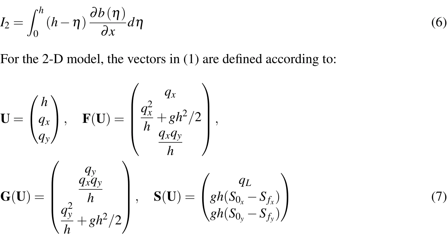
wherexandyare the spatial co-ordinates,qx,qythe unit discharges inx-andydirections,uandvthe velocities inx-andy-directions,qLthe lateral in flow.The friction slope is calculated according to:

Thegoverningequationsofthesystem(1)weresolvedusinga finitevolumemethod approach.In particular,equation(1)can be discretized as follows:

whereUiis the average value of the flow variables over the control volume Ωiat a given time;iandjrefer,respectively,to theith cell and thejth edge of the cell;kis the total number of the cell edges;nijand ΔΓijare the unit outward normal vector and the length of thejth edge respectively;E∗is the numerical flux through the edge which may be computed by an appropriate Riemann solver.

For both the models,the upwind Roe scheme[Roe(1981)]was used for computing the numerical fluxes.This choice was taken intentionally by the authors in order to minimize the differences due to the numerical solver.The presented models are able to solve the flood wave propagation in complex topographies.The upwind treatment of the source term is applied to the 1-D model[Petaccia,Natale,Savi,Velickovic,Zech,and Soares-Frazão(2013)]while the 2-D model uses state-ofthe-art techniques for source terms,friction slope and wet/dry fronts[Costabile and Macchione(2015)].For both the models presented,a semi-implicit treatment of the friction slopes is used in order to improve the stability of the numerical code[Petaccia,Natale,Savi,Velickovic,Zech,and Soares-Frazão(2013);Costabile,Costanzo,and Macchione(2013)].

The 2-D numerical scheme is based on the following key aspects:

a)an unstructured grid,generated using the Delaunay triangulation,has been used to obtain the computational domain composed by an irregular triangular network(TIN).Due to its high degree of flexibility and adaptability,an accurate geometrical description of the site can be provided even in the presence of signi ficant topographical gradient or when the hydraulic variables are expected to change very rapidly(hydraulic jump,shock wave and so on);

b)the bottom slopes were computed using the equation of the plane Z containing the three vertices of the triangles that cover the computation domain.The derivatives of Z over x and y give the bottom slopes along the two spatial directions;

c)due to the peculiarity of the computational domain(the bed is represented as a plane passing through the vertices of the cell),a cell can be dry,fully or partially wetted according to the free-surface water level(Y).The relationship between the water depth h in the barycenter of the triangle andY is trivial for fully wetted cells but it is not for partially wetted cells so the algebraic equations proposed by Begnudelli and Sanders(2007)were implemented.Moreover,a speci fic algorithm,inspired by Sleigh,Gaskell,Berzins,and Wright(1998),was used to manage the wet-dry fronts.In particular,the continuity equation is solved for all cells,while momentum equations are solved only if some pre-assigned conditions are ful filled:1)cell is fully wet;2)cell is partially wet but there is,at least,one neighbouring wet cell 3)cell is partially wet(letYpwthe associated free-surface water level)but there is,at least,a one neighbouring partially wet cell having free-surface water level higher thanYpw.

The 1-D numerical scheme is based on the following key aspects:

a)The system(1)is discretised over a domain divided into computational cells assuming constant values of the conserved variables A and Q over each cell.The variables are de fined here over an entire cell,as cell-averaged values;

b)An uncoupled formulation for the topographical source term is used.This term is discretised in a centered way:

where I2is calculated as the derivative of I1for a constant water depth hiaccording to equation(3).The spatial integration step is not constant.

c)If the cross section has a compound shape it is possible to de fine a global conveyance factor for the cross section based on the assumption that the friction slope is constant across the section width[Cunge,Holly,and Vervey(1980)].The conveyance of the compound cross section can be computed as:

whereNis the number of subsections andnMiis the Manning coef ficient of subsectioni.

3 Description of Crati and Corace River case studies

The cases here presented are located on the Crati River and the Corace River(Calabria region,in the South of Italy).A 0.5 m digital elevation model(DEM)was available for both case studies.

The study reach of Crati river has a mean slope of 1%.It is located just downstream the con fluence with the Busento river,where the Crati flows in the urban area of Cosenza(see figure 1).The overall length of the studied reach is about 10 km.The Europa bridge is located about 2 km downstream of the upstream boundary.

Figure 1:Overview of the bridge located on the Crati river

The study reach of the Corace river has a mean slope of 0.6%.It is located 8.7 km downstream of the upstream boundary,in the downstream part of the Corace basin and not far from the mouth in the Ionian sea(see figure 2).The total length of the studied reach is 13 km.

For both the study reaches,simulations presented here are based upon analysis of the 500-year discharge return frequency event,that is the most critical scenario prescribed by the Italian regulations.

Figure 2:Overview of the bridge located on the Corace river

4 Bridge analysis

In both the models,the bridges are represented in a different way.For the 1-D model,the distance between two consecutive cross sections is signi ficantly reduced near the bridges,in order to provide a reliable reconstruction of the bed pro file[Petaccia and Natale(2013)].The bridges are simulated considering four sections:the first two interior sections containing the piers obstructions and two other sections upstream and downstream of the bridge are added in order to correctly locate the narrowing induced by the piers themselves(see,for example, figure 3).For the 2-D model the bridges are added directly in the TIN.Piers are treated as solid wall conditions and added as internal boundaries(see for example figure 3).

5 Results and discussion

The 1-D and the 2-D models here presented were not calibrated since no detailed data of historical floods were available.For this reason,the compared analysis of 1-D and 2-D models aims at highlighting the backwater effects simulated by the two approaches using an assigned scenario.However,a speci fic procedure for reasonable estimations of roughness coef ficients was applied[Costabile,Macchione,Natale,and Petaccia(2015)].

As it is well-known,the water elevation simulated by the 1D model is constant across the section while this is not so for the 2-D model.In order to show the variability of the 2-D results along a 1-D cross section,the 2-D results are discussed with reference to two different axes.The 1-D river axis,referred to as “river axis”in the following,was chosen to represent the main channel during the flood.It does not represent the thalweg line and it was chosen by the authors in order to have 1-D cross sections perpendicular to it.A second axis,namely “axis 1”,was chosen to show the hydraulic phenomenon near the bank(see figure 3).

5.1 Europa bridge on the Crati River

The Europa bridge is placed 200 m downstream of the Busento con fluence(see figure 1).Upstream,there are two other bridges,approximately at a distance of 100 m,with piers in the main channel.

The bridge deck stands on three rectangular piers,whose dimensions are 3.2 m x 10 m.The river bed is con fined by arti ficial levees.The channel is quite regular,90 m wide.Three weirs are also located in this reach,located at x=2020 m,x=2160 m and x=2370 m( figure 4).

Figure 3 shows the bridge(piers in yellow),the cross sections used for the 1-D simulation(in yellow the sections describing the bridge)and the river axis of the 1-D model.The map of the flooded area by the maximum water depths simulated by the 2-D model is represented in figure 3.

5.1.1 2-D Analysis

The comparison between the solutions of the 2-D model,carried out with(“bridge”in figure 4)and without bridge piers(“no bridge”),is shown in figure 4.In particular,the bed levels along the river axis(z2D,RA),the maximum water surface(Y2D),the maximum total head(H2D)and the local Froude numberputed in a speci fic instant of time(approximately the water depth peak)for each triangular cell along the river axis of the 1-D model,are represented.

The bridge induces a backwater effect,whose length is about 20 m,that the 2-D model is able to reproduce,despite some slight diffusion in the solution.As shown in figure 4,the flow is supercritical approaching the bridge.The piers provoke a variation in the flow regime just upstream of the bridge(near the section 2150 m),which is not present if the piers are neglected,and then supercritical flow is restored.The simulation carried out without bridge highlights a supercritical flow along the river axis throughout the analyzed reach.The transition to supercritical flow occurs with a jump in the water pro file,con firmed by the local Froude number pro file(see figure 4,approximately x=2130 m).

The different transversal flow behavior is evident when analyzing the water surface level pro file near the river left bank,for example along the axis 1(see figure 3)that is located about 15 m from the bank itself.As shown in figure 5,in this area the incoming flow is supercritical in both the situations(with and without bridges).When the bridge is not represented,the flow regime turns to subcritical 60 m far from the bridge and no variation occurs along this axis up to the weirs downstream.

Figure 3:Europa bridge on the Crati river,cross-sections of the 1-D model and flood-prone areas simulated by the 2-D model represented as a contour map of the maximum water depths.

Flow behavior is similar considering the bridge.Therefore,while the 2-D water surface level pro file along the river axis highlights the typical variation of the flow regime provoked by the narrowing induced by the piers,the pro file extracted near the bank is always subcritical close to the bridge.As a consequence,a mixed flow regime(subcritical-supercritical)exists across the river cross-section.The different hydraulic behavior observed along the two axes can be explained since axis 1 covers a zone acting like an off-channel storage area,while river axis falls in the conveyance area.This interpretation is supported by the analysis of figure 6,where the total head and the water level are represented in a cross-section just upstream of the bridge(approximatelyx=2140 m)for a given instant of time near to the water depth peak value.PointsP1andP2,intersections between the crosssection and axis 1 and river axis respectively,are also highlighted.NearP1there are no signi ficant differences between the total head and water elevation.This means that the kinetic energy term is practically zero.The situation is completely different nearP2,where the difference between the two variables is consistent,con firming that axis 1 falls in the conveyance area.

In figure 7,the maximum water surface levels simulated with or without piers are represented in the same section as before.In the same figure,the bridge sof fit level and piers are also represented.Looking at the results,it may be noted that the maximum surface levels show signi ficant transversal variations with local water rise close to the piers.Considering the middle pier,water super elevation is almost two meters.This fact can be explained by the signi ficant reduction of the flow velocity upstream of the pier induced by the pier itself that acts as a solid wall.In fact,looking at the second opening in the left( figure 6),the difference between the two lines suddenly reduces close to the middle pier.As a consequence,the water level is forced to rise and this super elevation can be evaluated by computing the kinetic energy term,u2/(2 g),since the simulated velocity at the left of the middle pier is about 6 m/s.

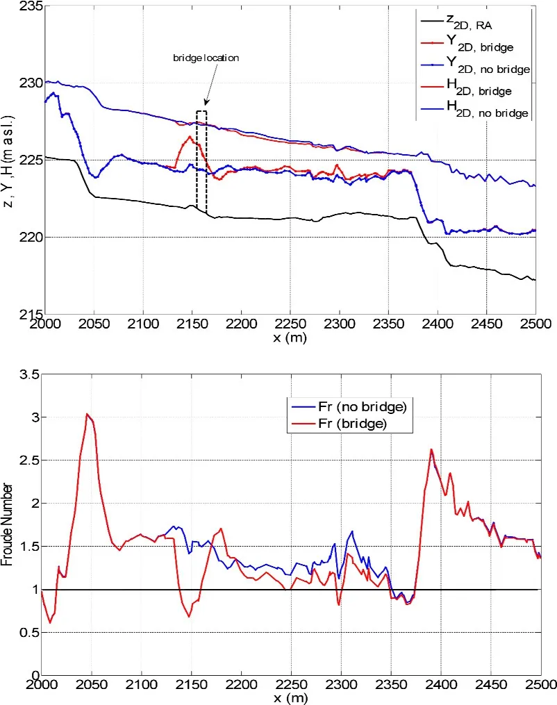
Figure 4:Maximum free-surface levels and maximum total head pro files along the river axis(above)and local Froude number pro file in a given instant of time(below)simulated by the 2-D model with and without piers.

For flood risk assessment,the percentage of the cross-section width,for which a given freeboard(for example 1 m)is ensured,is particularly interesting.It may be noted that in 65%of the cross-section width the freeboard of 1 m is ensured while the level of the maximum water rise,induced by the first pier on the right,is equal to 227 m a.s.l.,that is the same as the sof fit level.

Figure 5:Maximum free-surface levels and maximum energy pro files along axis 1(above)and local Froude number pro file(below)simulated by the 2-D model with and without piers

It should be stressed that what has been discussed above represents just one aspect of a detailed hydraulic bridge analysis.Indeed,besides the effect induced by piers,the role played by erosion,transport of sediments and debris should be taken into account in order to complete the analysis.

5.1.2 1-D Analysis

Figure 8 shows the comparison between the maximum water elevations and total head computed by the 1-D model with and without the bridge piers.

Figure 6:Total head and water elevations across the section x=2140 m simulated by the 2-D model(bridge scenario)

Figure 7:Maximum free-surface level for the section x=2140 m simulated by the 2-D model with and without piers.

Neglecting the bridge piers,the flow is supercritical in all the considered reach.The presence of the piers generates a hydraulic jump and a backwater effect of double extension if compared to the 2-D results.If the energy grade line is considered,the calculated total head may inaccurately increase owing to errors in computing water elevations and,mainly,water discharges.This may occur in very complex topography zones,in presence of weirs and narrowing sections[Petaccia,Natale,Savi,Velickovic,Zech,and Soares-Frazão(2013)].

To analyse in details the 1-D results,in figure 9 the comparison between the maximum 1-D water elevation computed with and without the bridge piers at the cross section just upstream the bridge is shown.Looking at the backwater pro file,the maximum level(226.26 m a.s.l.)is located near the bridge site.The hydraulic freeboard computed by the 1-D results is 0.76 m below the bridge sof fit,lower than the 1 m prescribed by some regulations.

The Italian Po river basin authority in 1999 issued the directive“Criteria for the assessment of the hydraulic compatibility of public infrastructures inside A and B regions”,where guidelines are de fined for bridge planning and management.It states that the minimum freeboard between the bridge sof fit and the water level corresponding to the design flood should not be less than 1 m and 0.5 times the kinetic energy.The freeboard has to be guaranteed for at least 2/3 of the bridge opening if the bridge is not linear,and in any case greater than 40 m.

The guidelines reported in the above recalled Directive refer,implicitly,to a 1-D hydraulic analysis for the evaluation of freeboard.

One of the main differences between the free-surface levels simulated by the models is due to the intrinsic limit of the 1-D model in reproducing the transversal variation across the section( figure 9).Therefore,the super elevations simulated by the 2-D models,due to the interaction with the piers,cannot be simulated by the 1-D approach.To overcome this limitation,the total head might be used as an indirect estimation of the maximum local super elevation.This expedient can be justi fied in part by the features of the 2-D simulation close to the piers.In particular,in the latter case it is expected that the kinetic energy is very small just upstream of the piers because of the obstacle induced by the piers themselves.However,as may be noted in figure 9,the total head of the 1-D model,used for the prediction of the maximum local water rise,overestimates the solution provided by the 2-D model by up to 60 cm.However,we must say that not even the 2-D calculation can give very accurate results,as 3D phenomena around the piers occur.

5.2 Bridge on the Corace River

The bridge is located in a river reach constrained by the topography on the right.On the left there is a wide floodplain of 270 m width that is,in turn,limited by the railway.The bridge is composed of two traf fic lanes and the two bridges stand very close together.There are four piers that might interact with the flow.The first three piers on the right have a circular shape whose diameter is 2.5 m.The last one is rectangular and its dimension is 2 m x 4 m.An overview of the bridge on the Corace river,its piers(in black),the cross-sections of the 1-D model as well as a representation of the flood-prone areas simulated by the 2-D model(2-D map representing the simulated maximum water depths)are shown in figure 10.

Figure 8:Longitudinal pro file of the maximum 1-D water elevation and total head with or without bridge piers

Figure 9:Comparison between the maximum computed 1-D and 2-D water elevations in the just upstream bridge section with or without the bridge piers

5.2.1 2-D analysis

Looking at the simulation carried out with piers,the 2-D model simulates the transitionthroughthecriticalstatenearthedownstreampiersthatinteractwiththemain channel flow( figure 11).In order to check if this effect is induced by the bridge,a simulation without piers has been carried out.Figure 11 shows that the transition through the critical state occurs also in this case,proving that this effect is simply due to the morphologic features of the river reach that has,in this part,a natural narrowing.The upstream pro file shows an increase of the water level up by to 10 cm.The length of backwater effect is about 200 m.

Figure 10:Bridge on the Corace river,cross-sections of the 1-D model and representation of the flood-prone areas simulated by the 2-D model.

The free-surface levels across the section just upstream of the first row of piers show local super elevations of water level due to the interaction between the flow and the single piers(see the arrows in figure 12).This effect is not extended across the section but it is located only in the areas immediately close to the piers.In conclusion,this bridge induces local effects in the cross-section water surface pro file,resulting in super elevations of the water just upstream of the piers.Therefore,the piers do not provoke the transition through the critical state but just a little increase of the backwater effect.Due to over flow upstream,some discharges propagate in off-channel area(see letter A in figure 10)explaining the water table on the left of figure 12(60 m＜y＜130 m).

5.2.2 1-D analysis

The 1-D model simulates the transition through the critical state on both cases(with and without piers)like the 2-D model,see figure 13.The simulated backwater effect has an extension of 200 m,comparable to the 2-D extension.

Figure 11:Maximum free-surface levels along axis 1(above)and local Froude number pro file at time-to-peak of water levels(below)simulated by the 2-D model with and without piers

The first bridge cross section is shown in figure 14,together with the maximum 1-D computed water elevations with or without the bridge piers.The computed backwater elevation is 0.43 m.The reasoning discussed in the analysis of the Europa bridge about a possible expedient to approximate the local super elevation of the water levels is re-proposed here.In this case,the total head value of the 1-D model is similar to the maximum water rise induced by the piers in the 2-D simulation.

6 Conclusions

Figure 12:Maximum free-surface level across the section just upstream of the bridge simulated by the 2-D model with and without piers

Figure 13:Longitudinal pro file of the maximum 1-D water elevation and total head with or without bridge piers

The authors presented a compared analysis of 1-D and 2-D flood propagation models in actual rivers with bridges.The models,based on the unsteady flow equations writteninconservativeform,werenotcalibrated,sincenodetaileddataofhistorical flooding were available.For this reason,the presented analysis aims at highlighting the backwater effects simulated by the two approaches using a given scenario.In particular,the two models were compared to analyse the effects of two bridges perpendicular to the flow along almost regular river reaches.Such a situation is usually treated using a 1-D schematization of the flow,assuming that the following hypotheses are ful filled:1)the flow regime is uniform on the cross section;2)the water elevation is horizontal across a section.

The cases here presented show signi ficant variations in water elevation on the cross section and a transversal regime transition within the cross section.These phenom-ena occur even in the first case here analyzed,although it is a classic example of rectangular narrowing cross section with rectangular piers.

Figure 14:Comparison between the maximum computed 1-D and 2-D water elevations in the bridge section with or without the bridge piers

The second case shows that considering a unique effect played by the bridge on flow dynamics can be misleading,even for a perpendicular bridge,since the effects of the piers need to be analyzed individually.

However,it has to be stressed that no uncertainty analysis was carried out,which might affect the presented analysis.

Moreover,it is important to emphasize that the results presented in this paper do not exhaust the subject of the flood hazard in presence of bridges:neither in general nor for the cases analyzed here.Indeed,besides the effect induced by piers,the role played by erosion and sediment transport of sediments and debris should be taken into account.

Acknowledgement:This work was supported in part by the European Union and the Region of Calabria in the funding project POR Calabria 2000-2006 Asse 1,Misura 1.4,Azione 1.4.c,“Studio e sperimentazione di metodologie e tecniche per la mitigazione del rischio idrogeologico”Lotto 8 “Metodologie di individuazione delle aree soggette a rischio idraulico di esondazione”.

Ali,A.M.;Di Baldassarre,G.;Solomatine,D.P.(2013):The impact of bridges on flood propagation and inundation modelling.Proceedings of the 35th IAHR World Congress,Chengdu,2013,Edited by:Wang Z.,Lee,J H-w,Gao J.,Shuyou,C.

Begnudelli,L.;Sanders,B.F.(2007):Conservative wetting and drying methodology for quadrilateral grid finite-volume models,Journal of Hydraulic Engineering,vol.133,no.3,pp.312–322.

Brandimarte,L.;Woldeyes,M.K.(2013):Uncertainty in the estimation of backwater effects at bridge crossings.Hydrological Processes,vol.27,pp.1292–1300.

Cao,Z.;Meng,J.;Pender,G.;Wallis,S.(2006):Flow resistance and momentum flux in compound open channel.Journal of Hydraulic Engineering,vol.132,pp.1272–1282.

Caviedes-Voullième,D.;García-Navarro,P.;Murillo,J.(2012):In fluence of mesh structure on 2-D full shallow water equations and SCS Curve Number simulation of rainfall/runoff events.Journal of Hydrology,vol.448–449,pp.38–59.

Cobaner,M.;Seckin,G.;Kisi,O.(2008):Initial assessment of bridge backwater usinganarti ficialneuralnetworkapproach.CanadianJournalofCivilEngineering,vol.35,pp.500–510.

Cook,A.;Merwade,V.(2009):Effects of topographic data,geometric con figuration and modeling approach on flood inundation mapping.Journal of Hydrology,vol.377,pp.131–142.

Costabile,P.;Macchione,F.(2012):Analysis of one-dimensional modeling for flood routing in compound channels.Water Resources Management,vol.26,pp.1065–1087.

Costabile,P.,Macchione,F.(2015):Enhancing river model set-up for 2-D dynamic flood modelling.Environmental Modelling&Software,vol.67,pp.89–107.

Costabile,P.;Costanzo,C.;Macchione,F.(2013):A storm event watershed model for surface runoff based on 2-D fully dynamic wave equations.Hydrological Process,vol.27,pp.554–569.

Costabile,P.;Macchione,F.;Natale,L.;Petaccia,G.(2015):Flood mapping using LIDAR DEM.Limitations of the 1-D modeling highlighted by the 2-D approach.Natural Hazards,vol.77,no.1,pp.181–204.

Cunge,J.A.;Holly,F.M.;Vervey,A.(1980):Practical aspects of Computational River Hydraulics.Pitman Publ.Inc,London.

Ernst,J.;Dewals,B.J.;Detrembleur,S.;Archambeau,P.;Erpicum,S.;Pirotton,M.(2010):Micro-scale flood risk analysis based on detailed 2-D hydraulic modeling and high resolution geographic data.Natural Hazards,vol.55,pp.181–209.

Fewtrell,T.J.;Neal,J.C.;Bates,P.D.;Harrison,P.J.(2011):Geometric and structural river channel complexity and the prediction of urban inundation.Hydrological Processes,vol.25,pp.3173–3186.

Gallegos,H.A.;Schubert,J.E.;Sanders,B.F.(2009):Two-dimensional,highresolution modeling of urban dambreak flooding:A case study of Baldwin Hills,California.Adv Water Resources,vol.32,pp.1323–1335.

Hailemariam,F.M.;Brandimarte,L.;Dottori,F.(2014):Investigating the influence of minor hydraulic structures on modeling flood events in lowland areas.Hydrological Processes,vol.28,no.4,pp.1742–1755.

Hunt,J.;Brunner,G.W.;Larick,B.E.(1999):Flow transitions in bridge backwater analysis.ASCE Journal of Hydraulic Engineering,vol.125,no.9,pp.981–983.

Kaatz,K.J.;James,W.P.(1997):Analysis of alternatives for computing backwater at bridges.ASCE Journal of Hydraulic Engineering,vol.123,no.9,pp.784–792.

Macchione,F.;Viggiani,G.(2004):Simple modelling of dam failure in a natural river.P I Civil Eng-Water Management,vol.157,pp.53–60.

Mantz,P.A.;Benn,J.R.(2009):Computation of af flux ratings and water surface pro files.Proceedings of the Institution of Civil Engineers Water Management,vol.162,no.WM1,pp.41–55.

Martin-Vide,J.P.;Prio,J.M.(2005):Backwater of arch bridges under free and submerged conditions.Journal of Hydraulic Research,vol.43,no.5,pp.515–521.Morales-Hernandez,M.;Petaccia,G.;Brufau,P.;Garcia Navarro,P.(2015)Conservative 1D-2D coupled numerical strategies applied to river flooding:the Tiber(Rome),accepted for publication inApplied Mathematical Modelling

Pappenberger,F.;Matgen,P.;Beven,K.J.;Henry,J.B.;P fister,L.;De Fraipont,P.(2006):In fluence of uncertain boundary conditions and model structure on flood inundation predictions.Advances in Water Resources,vol.29,pp.1430–1449.

Petaccia,G.;Natale,E.(2013):ORSADEM:a one dimension shallow water code for flood inundation modeling.Journal of Irrigation and Drainage,vol.62,no.2,pp.29–40.

Petaccia,G.;Natale,L.;Savi,F.;Velickovic,M.;Zech,Y.;Soares-Frazão,S.(2013):Flood wave propagation in steep mountain rivers.Journal of Hydroinformatics,vol.15,no.1,pp.120–137.

Picek,T.;Havlik,A.;Mattas,D.;Mares,K.(2007):Hydraulic calculation of bridges at high water stages.Journal of Hydraulic Research,vol.45,no.3,pp.400–406.

Ratia,H.;Murillo,J.;García-Navarro,P.(2014):Numerical modeling of bridges in 2D shallow water flow simulations.International Journal for Numerical methods in fluids,vol.75,pp.250–272.

Roe,P.L.(1981):Approximate Riemann Solvers,parameter vectors and difference schemes.Journal of Computational Physics,vol.43,pp.357–372.

Seckin,G.;Haktanir,T.;Knight,D.W.(2007):A simple method for estimating flood flow around bridges.Proceedings of the Institution of Civil Engineers Water Management,vol.160,no.WM4,pp.195–202.

Sleigh,P.A.;Gaskell,P.H.;Berzins,M.;Wright,N.G.(1998):An unstructured finite volume algorithm for predicting flow in rivers and estuaries.Computers&Fluids,vol.27 no.4,pp.479–508

1LAMPIT,Laboratorio di Modellistica Numerica per la Protezione Idraulica del Territorio,Department of Environmental and Chemical Engineering,University of Calabria,Italy

2Department of Civil Engineering and Architecture,University of Pavia,Italy