Randomly Weighted LAD-Estimation for Partially Linear Errors-in-Variables Models

Xiaohan YANG Rong JIANG Weimin QIAN

1 Introduction

Consider a partially linear errors-in-variables(EV for short)model as follows:

where xi∈ Rpare unobservable explanatory variables,Xi∈ Rpare manifest variables,β0∈ Rpis an unknown parameter vector,Tiis a scalar co-variate,the function g(·)is unknown,Yi∈ R are responses,and(ε,uT)T∈ Rp+1are independent with a common error distribution that is spherically symmetric.Spherical symmetry implies that εiand each component of uihave the same distribution,which ensures model identi fiability and means that(ε,uT)T=dRUp+1(R is a nonnegative random variable,Up+1is a uniform random vector on Ωp={a:a ∈ Rp+1,‖a‖=1},R and Up+1are independent),and(ε,uT)Tand x are independent.A detailed coverage of linear errors-in-variables models can be found in[7].More work on nonlinear models with measurement errors can be found in[2].Recently,the model(1.1)has been studied by Cui and Li[5],Liang et al.[13],Zhu and Cui[24]and so on.Cui and Li[5]and Liang et al.[13]discussed the least square estimators for the parametric and nonparametric components by the nearest neighbor estimation and the general kernel smoothing for the nonparametric component,respectively.The quantile estimate of the slope parameter β0has been studied by He and Liang[8].

It is well known that the least square(LS for short)method is one of the oldest and most widely used statistical tools for linear models.But,the LS estimate can be sensitive to outliers and therefore,non-robust.Unlike the LS method,the least absolute deviation(LAD for short)method is not sensitive to outliers and produces robust estimates.Due to the developments in theoretical aspects and the availability of computing power,the LAD method has become increasingly popular.In particular,it has many applications in econometrics and biomedical studies(see[1,10]),among many others.

However,the asymptotic distribution of the estimators by the LAD method is generally related to nuisance parameter that can not be conveniently estimated.The randomly weighted method can provide a way of assessing the distribution of the estimators without estimating the nuisance parameter.The random weighting method was first proposed by Zheng[23].An advantage of the random weighting method is that no observation is repeatedly used within each replicate of the random weighting,though each observation may be weighted unequally.This method has been used in many applications as an alternative to the bootstrap method.For example,Rao and Zhao[16]used this method to derive the approximate distribution of the M-estimator in the linear regression model.Cui et al.[6]proposed a random weighting method for the proportional hazards model.Wang et al.[19]extended the method to the censored regression model.Jiang et al.[9]discussed randomly weighted least square estimators for the unknown parameters in semi-linear EV model.A statistical analysis of the LAD method used in the partially linear regression model(1.1)with additive measurement errors,however,still seems to be missing.The objective of the present paper is to fill this gap.

In this paper,our objective is to apply the randomly weighted LAD-estimation(RWLADE for short)to partially linear EV models,and establish the asymptotic normality of the RWLADE for the parameter.These results can be used to construct confidence intervals for β0.Furthermore,we propose a LAD-test for partially linear EV models.The LAD-test has been used by Zhao and Chen[22]to test linear hypotheses in the linear model.But the critical values of the test statistic are related to estimators of nuisance parameters.Chen et al.[3]proposed an easy and convenient randomly weighting resampling method to determine the critical values for testing linear hypotheses in the least absolute deviation regression.Motivated by this idea,we also use the randomly weighted method to determine the critical values for testing hypotheses in partially linear EV models.

The outline of the paper is as follows.In Section 2,we define the weighting scheme to be used,hence the RWLADE for β0,and then the test statistics of it.Section 3 is the statement of the main results for β0,and the chi-square distributions of test statistics of the proposed estimators are also given in this section.In Section 4,simulations are carried out to assess the finite sample performance of the method and also an illustration of the method to a real example is given in this section.Some concluding remarks are given in Section 5.All the technical proofs are delayed in the appendix of Section 6.

2 Definition of the Estimators

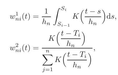
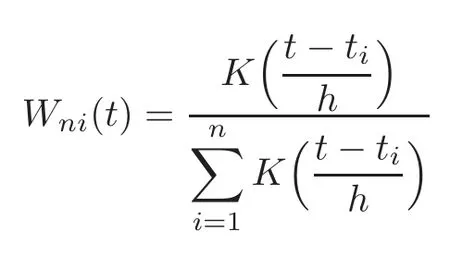
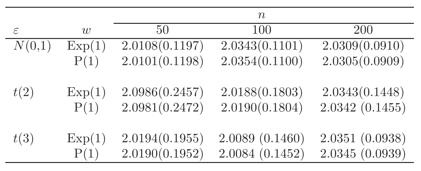
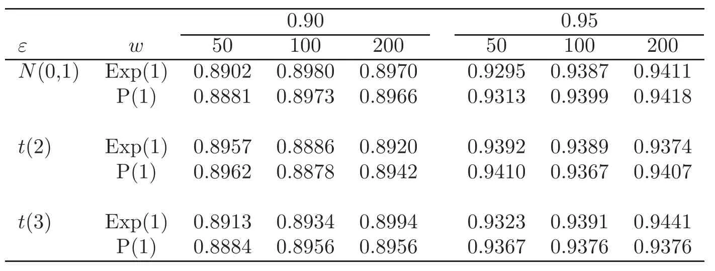
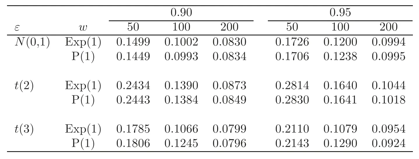
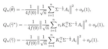
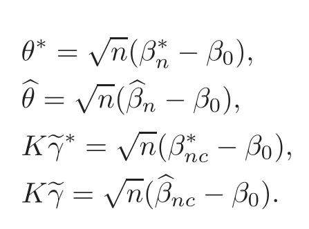
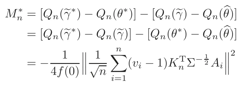
For technical convenience we will assume that Tiare con fined to the interval[0,1].Throughout,we shall employ a constant C(0

For any t∈ [0,1],we arrange|T1−t|,|T2−t|,···,|Tn−t|in an increasing order:

(ties are broken by comparing indices).Obviously,R(1,t),R(2,t),···,R(n,t)is a permutation of{1,2,···,n}.Choose a group of fixed nonnegative numbers{dni:i=1,2,···,n}and let k ≡ knbe a natural number dependent solely on n.Suppose that{dni:i=1,2,···,n}and k satisfy

Now we can define a probability weight vector wni(t)=wni(t;T1,T2,···,Tn),i=1,2,···,n which satisfies wnR(i,t)(t)=dni,i=1,2,···,n.Obviously,1 ≤ dni≤ n,1 ≤ wni(t)≤ n for any i=1,2,···,n,t∈ [0,1].These assumptions are commonly assumed when de fining weight nonnegative functions.For example,

where Si=(T(i)+T(i−1)),i=1,···,n,S0=0,Sn=1 for any i=1,2,···,n,t∈ [0,1].

In this paper,for any sequence of variables or functions(S1,···,Sn),we always denote ST=(S1,···,Sn),andThe conversion from S towill be applied to Yi,Xi,xi,εi,uiand g(Ti).For example,Xi−The fact that g(t)=E(Yi−|Ti=t)suggests

as the nearest neighbor pseudo-estimator of g(·).

However,since β0is an unknown vector,we have to estimate β0first.Sinceare unobservable,the least square method may be invalid.Instead of the generalized least square method used in[5],we can obtainthe estimator of β0,as follows:

But the asymptotic covariance matrix ofinvolves the density of the errors and nuisance parameters and therefore is difficult to estimate reliably.To overcome this problem,we propose the following distributional approximation based on random weighting by exogenouslygenerated i.i.d.random variables.The approach can be implemented with the simple LAD programming again.

Let v1,···,vnbe a sequence of independent and identically distributed(i.i.d.)nonnegative random variables,with mean and variance both equal to 1.The standard exponential distribution has mean and variance equal to 1.define

In this paper,we are also interested in testing the hypothesis

where H is a known p×q matrix of rank q,and b0∈Rpis a known vector(0

To develop an analogue with the least absolute deviation,it is natural to consider the test statistic

where

But the limiting distribution of Mnalso involves the density function of the error terms.Chen et al.[3]proposed an easy and convenient randomly weighted resampling method to determine the critical values for testing nested linear hypotheses in the least absolute deviation regression.Motivated by this idea,we introduce a test statistic M∗non randomly weighted method and on the suitable centering adjustments.The approach can be implemented with the simple LAD programming again.define

where

3 Main Results

Let the components be xi=(xij).Denote hi=(hi1,hi2,···,hip)T=xi− E(xi|Ti),1 ≤i≤n.We make the following assumptions.

Assumption 3.1the random weights v1,···,vnare i.i.d.with P(vi≥ 0)=1,E(vi)=Var(vi)=1,and the sequence viand Yi,Xi,xiare independent.

Assumption 3.2the distribution function F of ε1,···,εnis absolutely continuous,with continuous density f uniformly bounded away from 0 and∞and F(0)=.

Assumption 3.3ER2<+∞and P(R=0)=0.

Assumption 3.4The distribution of T1is absolutely continuous and its density r(t)satisfies

Assumption 3.5Σ =Cov(x1−E(x1|T1))is a positive de finite matrix.

Assumption 3.6E(|ε1|2+‖x1‖2+‖u1‖2)< ∞;g and g2jare continuous functions on the interval[0,1],where g2j=E(x1j|T1=t)is the jth component of g2(t)=E(x1|T1=t)for 1≤j≤p.

Assumption 3.7E(|ε1|4+‖x1‖4+‖u1‖4)< ∞;g and g2jsatisfy the Lipschitz condition and g2j=E(x1j|T1=t)is a bounded function of t for 1≤j≤p.

Remark 3.1Assumption 3.1 is commonly assumed in the random weighting method(see[19]).Assumptions 3.2–3.3 are often used in the LAD estimator(see[4,H1–H4]).Assumptions 3.4–3.6 are necessary for studying the optimal convergence rate of the nonparametric regression estimates and Assumption 3.7 guarantees the asymptotic normality of√n(−β),essentially the same as the conditions 1–4 of[5].

3.1 Random weighting LAD-estimation

Theorem 3.1Suppose that Assumptions 3.1–3.7 and(2.2)–(2.3)hold,and then

Particularly,when vi≡1,we have

where

Theorem 3.2Suppose that the conditions of Theorem 3.1 hold,and then

Comparing(3.1)with(3.3),for the multivariate Kolmogorov-Smirnov distance betweenandwe have

where L∗,P∗denote the corresponding distribution and probability conditionally on(X1,Y1,T1),···,(Xn,Yn,Tn).And the approximate to the distribution ofby using random weights is valid in the weak sense.

Remark 3.2From Theorems 3.1–3.2,it is clear thatis a consistent estimator of β0and the conditionally limiting distribution offor observations given is the same as that ofConsequently,we can take the conditional distribution ofas an approximation to that ofwithout estimating the asymptotic covariance matrix when making the confidence interval for parameters.In practical applications,this can be done by the Monte Carlo method.Speci fically,one can generate random weights repeatedly for(2.6)and then obtain RWLADE of the regression parameters.Then the empirical distribution of the produced estimates is used as an approximation to the distribution of the LAD-estimator of β0.For example,in deriving the(1 − α)100%confidence interval for β0,one can implement the random weighting N times to obtain the estimates,···,and hence use the lower and upperquantiles of these quantities as the approximation of the lower and upper limits of the confidence interval.

3.2 LAD-test

Theorem 3.3Suppose that the conditions of Theorem 3.1 hold,and under the null hypothesis(2.4),then

where Hn=H(HTΣH)−12,Ai=and

where“”denotes approximation to the corresponding distribution,S=

3.3 Random weighting LAD-test

Theorem 3.4Suppose that the conditions of Theorem 3.1 hold,and under the null hypothesis(2.4),then

and

Further by(3.6)–(3.7),we have

where Z is the chi-squared variable with q degrees of freedom.

Remark 3.3Theorems 3.3–3.4 show that the limiting distribution ofunder the null hypothesis(2.7)is the same as the null limiting distribution of Mn.Therefore,we can directly use the conditional distribution ofas an approximation to the null distribution of Mnand determine the critical values of the test statistic Mnwithout estimating the nuisance parameters.It is desired to determine a sequence cn(α)such thatP(Mn>cn(α))= α under H0,for a given level α ∈ (0,1).As shown in the sequel,the(1 − α)quantile(α)of the conditional distribution offor givencan be taken as an approximation to cn(α),and this can be carried out by the following procedure.Take N large enough and generate N independent replicates of random weights to obtain N randomly weighting estimates,j=1,···,N,so then the p-value of testing the hypothesis is approximately equal to ♯ {j:>Mn,j=1,···,N}/N.A test at the nominal signi ficance level α is to reject H0if Mnis larger than the sample(1−α)quantile ofand to accept H0otherwise.It is easy to show that,for the given nominal signi ficant level α∈(0,1),the test Mnwith the critical value(α)has the same asymptotic level and asymptotic power as the test with the critical value cn(α)obtained by estimating nuisance parameters.

4 Simulation and Real Data Study

In this section,we conduct simulation studies to assess the finite sample performance of the proposed procedures and illustrate the proposed methodology on AIDS clinical trials.

Example 4.1The data are generated from model(1.1),where the explanatory variable x is generated from uniform distribution on the interval(3,5)and β0=2. ε ∼ N(0,1),u ∼N(0,1),g(t)=sin(2πt),T ∼ U(0,1).The randomly weighting variables viare taken to be exponential distribution and Poisson distribution with means 1 respectively(Exp(1)and P(1)).We use the Nadaraya-Watson kernel K(u)=I(|u|≤1);and then

is the weight function with the bandwidth h=Since the objective is to estimate β0,our limited experience indicates that the choice of the bandwidth h here is not as critical as it is in direct nonparametric function estimation.Sample size n is taken to be 50,100 and 200,respectively,and we do 500 repetitions for each sample size.The number of randomly weighting is N=500.

We first study the performance of parameter estimators by using our proposed method(RWLADE for short).The mean values of parameter estimators and their standard errors are respectively reported in Table 1.Table 1 shows that the performance ofis very close to the true value in all terms.Moreover,is much more accurate when sample sizes increase.

Table 1 Simulation results for β∗

We then investigate the length of confidence intervals and empirical coverage rates by the randomly weighted method at the nominal levels 90%and 95%.Simulation results are respectively reported in Tables 2–3.From Table 2,it can be seen that the empirical coverage rates are reasonably close to the true values in all cases,which indicates that the randomly weighted method is valid.As expected,the coverage levels based on the di ff erent cases are much closer to the nominal levels when sample sizes increase.Table 3 shows that the length of confidence intervals is small.Not unexpectedly,the length of confidence intervals decreases with sample sizes.Finally,Tables 1–3 show that the performances of Poisson weights are exactly similar to those of exponential weights.

Table 2 Simulation results for coverage probability of confidence intervals

Next,the approximation of the null distribution of the LAD-test statistics Mn,by its randomly weighted version,is evaluated under the null hypotheses.We also study the empirical signi ficance level and the powers of the M-test with the critical values given by the random weighting method.Throughout our simulation study,the convex function is taken as ρ(u)=|u|.The null hypothesis isH0:β0=0.Here,the randomly weighted variables are only taken to be the exponential distribution with means 1.

Table 3 Simulation results for length of confidence intervals

Table 4 lists the power functions at signi ficance levelsα=0.10 and 0.05 for various choices of error distributions(N(0,1),t(2)andt(3)),di ff erent sample sizesn=100 and 200,and di ff erentβvalues 0,0.1,0.2 and 0.5.Note that the empirical signi ficant levels when the trueβ=0 are close to the nominal levels,implying that the randomly weighted LAD-test is a valid test.As expected,the test has a bigger power for the larger sample sizes.

Table 4 Empirical signi ficant levels and power values

Figure 1 shows quantile-quantile plots ofMnwith respect tofor various choices of error distributions(N(0,1),t(2)andt(3)),and di ff erent sample sizesn=100 and 200,in which the straight lice indicates thatapproximates well to the distribution ofMn.It shows that,when the sample size is increased from 100 to 200,the distribution approximation for the larger size is much more accurate than that for the small one.

Example 4.2In this section,we model the relationship between viral load and CD4+cell counts in HIV-infected individuals during potent antiviral treatments based on the data from ACTG 315 study.In general,it is believed that the virologic response RNA(measured by viral load)and immunologic response(measured by CD4+cell counts)are negatively correlated during antiviral treatment(see[12,21]).And also the discordance between virologic and immunologic responses has been observed from several recent clinical studies(see[14–15,17,20])which model the relationship between viral load and CD4+cell counts by the mixed-e ff ect varying-coefficient model based on these data.In their studies,exact tests and confidence intervals for parameters are not available.Instead,we present these analysis results by model(1.1).Here,we also focus on the data for the first 24 weeks of treatment,since virological or immunologic responses during this period are popular endpoints for many AIDS clinical trials.So both viral load and CD4+cell counts were scheduled to be measured on days t=0,2,7,10,14,28,56,84,168 after initiation of an antiviral therapy.We obtained 441 complete paries of viral load and CD4+cell count observations from 48 evaluable patients.Let Yibe the viral load and let xibe the CD4+cell count for subject i.To reduce the marked skewness of CD4+cell counts and to make treatment times equal space,we take log-transformations of both variables(this is commonly used in AIDS clinical trials(see[14])).The xiare measured with error.The model we used is

Y= β0+xβ1+g(T)+ε,X=x+u,

where X is the observed CD4 cell counts and T is time.

Figure 1 Q-Q plot ofv.s.Mn

The parameter estimators,by using our proposed methods,are(β0,β1)=(2.7234,−0.1301).The 95%confidence interval of β0is(2.6496,2.7924)and that of β1is(−0.1498,−0.1085).It can be seen that the length of confidence intervals is small.Furthermore,we test the linear hypothesis H0:β1=0.The resulting p-value is 0,suggesting that β1is signi ficant.

5 Discussion

The primary goal of this paper is to provide a convenient inference and a linear hypothesis testing for the partially linear EV model based on the LAD-estimate.The proposed inference procedure via resampling avoids the difficulty of density estimation and is convenient to implement with the availability of the standard linear programming and computing power.All simulation studies con firm that the performance of the random weighting method works well.We believe that the proposed statistical method is methodologically valuable.Some of the conditions assumed for the main results may be dropped or relaxed and,in particular,the samples usually may not be independent in many applications.In addition,it allows that the LAD can be extended to the M method,and the random weighting method can be used in other nonparametric regression models,such as the mixed-e ff ect varying-coefficient model for AIDS data;the censored model or longitudinal data,which are common in survival analysis,and they are valuable subjects for future research.

6 Appendix

To prove the theorem,we first introduce the following three lemmas.

Lemma 6.1(1)Suppose that Assumption 3.6 and(2.2)–(2.3)hold,and then

(2)Suppose that(2.2)–(2.3)hold,E(|ε1|l+‖x1‖l+‖u1‖l)< ∞,and g and g2jsatisfy the Lipschitz condition.Then

for l=3 or 4.

ProofThis result is due to Lemma 1 of[5].

Lemma 6.2(1)Assume that Assumption 3.2 holds and that f is a continuous function on interval[0,1],andThen

(2)Assume that Assumption 2.2 holds and that f satisfies the Lipschitz condition and(n→∞).Then

ProofThis result is due to Lemma 2 of[5].

Lemma 6.3Under the condition of Theorem 3.1,we have

ProofObserve that xi=hi+g2(Ti),1≤i≤n,and we have

By virtue of Lemmas 6.1–6.2 and the strong law of large numbers,we have

and therefore,

so

Next we proceed to prove the theorems.

Proof of Theorem 3.1In this section,for simplicity in notation,let θ = √n(β − β0).

Write

By virtue of Lemmas 6.1–6.2 and the strong law of large numbers,we have

By applying the identity in Knight[11],

We have

Qn(θ)=Qn1(θ)+Qn2(θ),

where

Since

where=dstands for obeying the same distribution,we have

EQn2(θ)=EQn(θ)− EQn1(θ)

By the Schwarz’s inequality and the control limited theorem,it is easy to see that

and Assumption 3.2 then implies that

The convextiy of the limiting objective function Q0(θ)assures the uniqueness of the minimizer and consequently

Furthermore,

where

particularly,when v1≡1,we have

By the central limited theorem,we have

Proof of Theorem 3.2By the result of Theorem 3.1,we have

From Lemma 2.9.5 in[20],it follows that conditionally on

for almost every sequenceThus,by(6.12)–(6.13),it is easy to show that(3.3)holds true,

By using the similar argument as in[16],(3.4)can be shown to hold true.

Proof of Theorem 3.3define K as a known p×(p−q)matrix of rank p−q(0

and then

and

Without loss of generality,H0:HT(β −b0)=0 can be written as

β−β0=Kγ

for some γ ∈Rp−q,so

Let vi≡1.By Theorem 3.1,we have

It thus follows that

Replacing(6.14)into(6.15),we get

Similarly

whereWhen H0is true,

Under the condition of Theorem 3.3.This means that the Lindeberg’s condition holds.Moreover,note that

Proof of Theorem 3.4Similar to the proof of Theorem 3.3,define

and replacing into Qn(θ∗),we have

Similarly,it is easy to show that

So

where

Therefore

From Lemma 2.9.5 in[18],it follows that conditionally on

AcknowledgementThe authors are extremely grateful to the referees for their valuable comments and suggestions.

[1]Buchinsky,M.,Recent advances in quantile regression models:A practical guideline for empirical research.Journal of Human Resources,33,1998,88–126.

[2]Carroll,R.J.,Ruppert,D.and Stefanski,L.A.,Nonlinear Measurement Error Models,Chapman and Hall,New York,1995.

[3]Chen,K.,Ying,Z.and Zhang,H.,Analysis of least absolute deviation,Biometrika,95,2008,107–122.

[4]Cui,H.J.,Asymptotic properties of generalized minimum L1-norm estimates in EV model,Science in China,Series A,27,1997,119–131(in Chinese).

[5]Cui,H.J.and Li,R.C.,On parameter estimation for semi-linear errors-in-variables models,Journal of Multivariate Analysis,64,1998,1–24.

[6]Cui,W.Q.,Li,K.and Yang,Y.N.,Random weighting method for Cox’s proportional hazards model,Science in China,Series A,51,2008,1843–1854.

[7]Fuller,W.A.,Measurement Error Models,John Wiley and Sons,New York,1987.

[8]Hardle,W.,Liang,H.and Gao,J.T.,Partially Linear Models,Physica-Verlag,Beilin,2000.

[9]Jiang,R.,Qian,W.M.and Zhou,Z.G.,Randomly weighted estimators for parametric component in semi-linear errors-in-variables models,Journal of Tongji University,Natural Science,39,2011,768–772(in Chinese).

[10]Jin,Z.,Ying,Z.and Wei,L.J.,A simple resampling method by perturbing the minimand,Biometrika,88,2001,381–390.

[11]Knight,K.,Limiting distributions for L1regression estimators under general conditions,Ann.Stat.,26,1998,755–770.

[12]Lederman,M.M.,Connick,E.and Landay,A.,Immunologic responses associated with 12 weeks of combination antiretroviral therapy consisting of zidovudine and ritonavir:Results of AIDS clinical trials group protocol 315,The Journal of Infectious Diseases,178,1998,70–79.

[13]Liang,H.,Hardle,W.and Carroll,R.J.,Estimation in a semiparametric partially linear errors-in-variables model,Annual Statistics,27,1999,1519–1535.

[14]Liang,H.,Wu,H.L.and Carroll,R.J.,The relationship between virologic and immunologic responses in AIDS clinical research using mixed-e ff ect varying-coefficient semiparametric models with measurement error,Biostatistics,4,2003,297–312.

[15]Mallolas,J.,Li,W.and Del,R.A.,Clinical Outcome,CD4+Cell Count,and HIV-1 Reverse Transcriptase and Protease Sequences in Patients Remaining Viremic during HAART,7th Conference on Retroviruses and Opportunistic Infections,Abstract♯334,Jan 30-Feb 2,San Francisco,CA,2000.

[16]Rao,C.R.and Zhao,L.C.,Approximation to the distribution of M-estimates in linear models by randomly weighted bootstrap,SankhyA,54,1992,323–331.

[17]Sabin,C.,Staszewski,S.and Phillips,A.,Discordant Immunological and Virological Responses to HAART,7th Conference on Retroviruses and Opportunistic Infections,Abstract♯333,Jan 30-Feb 2,San Francisco,CA,2000.

[18]Van der Vaart,A.W.and Wellner,J.A.,Weak Convergence and Empirical Processes,Springer-Verlag,New York,1996.

[19]Wang,Z.,Wu,Y.and Zhao,L.C.,Approximation by randomly weighting method in censored regression model,Science in China Series A,52,2009,561–576.

[20]Wu,H.,Connick,E.and Kuritzkes,D.R.,Cell Kinetic Patterns and Their Relationships with Virologic Responses in HIV-1-Infected Patients Treated with HAART,7th Conference on Retroviruses and Opportunistic Infections,Abstract♯340,Jan 30-Feb 2,San Francisco,CA,2000.

[21]Wu,H.and Ding,A.,Population HIV-1 dynamics in vivo:Applicable models and inferential tools for virological data from AIDS clinical trials,Biometrics,55,1999,410–418.

[22]Zhao,L.C.and Chen,X.R.,Asymptotic behavior of M-test statistics in linear models,Journal of Combine Information System Science,16,1991,234–248.

[23]Zheng,Z.G.,Random weighting method,Acta Mathematicae Applilcate Sinica,10,1987,247–253(in Chinese).

[24]Zhu,L.and Cui,H.J.,A semiparametric regression model with errors in variables,Scan.Journal Statistics,30,2003,429–442.