Introducing robustness in model predictive control with multiple models and switching

Sachin PRABHU,Koshy GEORGE2,†

1.Department of Telecommunication Engineering,PES Institute of Technology,Bangalore 560085,India;

2.PES Centre for Intelligent Systems,Bangalore 560085,India

Introducing robustness in model predictive control with multiple models and switching

Sachin PRABHU1,Koshy GEORGE2,1†

1.Department of Telecommunication Engineering,PES Institute of Technology,Bangalore 560085,India;

2.PES Centre for Intelligent Systems,Bangalore 560085,India

Model predictive control is model-based.Therefore,the procedure is inherently not robust to modelling uncertainties.Further,a crucial design parameter is the prediction horizon.Only offline procedures to estimate an upper bound of the optimal value of this parameter are available.These procedures are computationally intensive and model-based.Besides,a single choice of this horizon is perhaps not the best option at all time instants.This is especially true when the control objective is to track desired trajectories.Inthis paper,we resolve the issue by atime-varying horizon achieved by switching between multiple model-predictive controllers.The stability of the overall system is discussed.In addition,an introduction of multiple models to handle modelling uncertainties makes the overall system robust.The improvement in performance is demonstrated through several examples.

Receding horizon control;Time-varying horizon;Multiple models;Switching;Tracking;Robustness

1 Introduction

Receding horizon control(RHC)or model predictive control(MPC)is perhaps the only control technique that has dominated in industrial control for several decades with thousands of applications.This is primarily due to its unique ability to handle rather effectively and in a simple manner the hard constraints on the states and control inputs.Constraints are natural in nearly all applications.For example,safety limits the values of variables such as temperature and pressure,and actuators saturate.RHC is based on the principle of determining online at each sampling instant k an open-loop control sequence over a finite-horizon.This sequence is typically computed at each instant by solving an open-loop optimization problem that is initialized with the current state of the industrial process or dynamical system to be controlled.The first element of the computed control sequence is the input to the plant at instant k and the remaining elements of this sequence usually discarded.This process is repeated at the next time instant k+1 over a shifted horizon based on new measurements.The optimizingprocedure involves the prediction of system behaviour over a finite-horizon in the future based on forward simulation of a mathematical model of the plant.This paves the way to easier dynamical handling of the input and state constraints.Naturally,MPC is highly sensitive to parametric variations and modelling uncertainties.

The seminal ideas of MPC have been proposed by several researchers[1,2].Advocated by the authors of dynamic matrix control in[3]and[4],the strategy became popular in the petro-chemical industry.Several variants of MPC have been proposed that differ in the plant and disturbance models,and the manner of adaptation in the case of time-varying models[5].The issues with MPC include the existence of a solution and its region of validity,closed-loop stability,and robustness towards parameter variations.Closed-form solutions to MPC are impossible as the constraints are to be handled dynamically.Accordingly,analyzing the stability of the closed loop with a receding-horizon type control is far from trivial.Robustness issues in unconstrained optimal control were addressed using internal model control[6–8].Generalized predictive control using input-output models was introduced in[9]and[10]to overcome the lack of robustness in self-tuning regulators.This was extended to state-space models in[11].Conditions for closedloop stability were derived in[12]and[13].In-depth reviews of MPC techniques and associated issues such as the existence of a solution and the region of validity of this solution,stability,and robustness feature in[14]and[15].

Though addressing constraints is easier with MPC than with any of the infinite-horizon optimal control techniques,it provides only an approximation to the global optimal solution.The length of the prediction horizon,which is a crucial design parameter in MPC,affects the accuracy of this approximation and closedloop stability of the overall system.Evidently,it influences as well the performance of MPC.Methods to choose this parameter optimally,and its implications on performance and stability,are discussed in[16–18].Techniques applicable to infinite-dimensional systems are treated in[19]and[20],and the possibility of reducing the prediction window size further with minimal compromise in performance discussed in[21]and[22].All these techniques attempt to obtain the best estimate for the optimal prediction window size;these are based on offline computations and are applicable to stateregulation problems.However,they are neither simple in practice nor precise.Even for finite-dimensional linear time-invariant(LTI)systems,it is possible to arrive at different estimates of this parameter using the method suggested in[18].Thus,choosing online an optimal prediction horizon is potentially an open problem.

The goal of this paper is to propose a receding-horizon type control based on multiple models and switching.Switching ensures a time-varying horizon resulting in an improvement in the time-domain performance relative to conventional MPC.Robustness to modelling uncertainties is introduced using multiple models.In this paper,we show that the proposed technique can be applied to the problems of regulation and set-point tracking,and tracking a class of reference trajectories despite modelling uncertainties.This paper extends the ideas proposed earlier in[23–25].

Tracking a non-zero constant reference can be addressed as a regulation problem by redesigning MPC with a suitable change in coordinates.A redesign of MPC whenever the desired set-point changes is a tedious process,and is impractical for rapidly varying set-points or arbitrary references.In order to overcome this problem,reference governors were introduced in[26]and[27]to modulate the reference signals to obtain artificial reference signals.Alternatively,a new optimization variable to approximate the original reference in an admissible way is introduced in[28]and[29].MPC designed for regulation is then used by both methods to ensure that the output tracks such admissible artificial reference signals.

Switching to improve performance is not new in MPC.For instance,switching between robust control and RH-type control is considered in[30–32].The effect of switching in a switched multi-objective MPC setup was analyzed in[33],where the switching signal is known a priori.These algorithms focus on improving the robustness and performance with MPC.A simple method to automatically arrive at a prediction horizon that is optimal at every instant of time by switching between multiple RH-type controllers was proposed in[23]for the regulation problem.The potential of such a switching technique to improve the transient performance was demonstrated whereas the stability issue was not addressed there.Whilst disturbance rejection was considered in[24],tracking of varying set-points was dealt with in[25].This paper introduces multiple models to make the overall system robust to a class of modelling uncertainties.

MPC is discussed in detail in Section 2.The computation of the control law together with its formulation as a quadratic program is described.The technique to introduce a time-varying horizon is dealt with here,and is achieved by switching based on a simple decision criterion.This eliminates laborious offline computational efforts required to optimally choose the prediction horizon.This is followed by a description of how multiple models are used to make the control law robust to modelling uncertainties.The performance of the proposed technique is compared with conventional MPC through experiments conducted on six systems.These simulation results are presented in Section 3.

2MPC

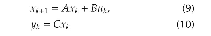
Consider a linear time-varying(LTV)system Σ with the following state-space description:

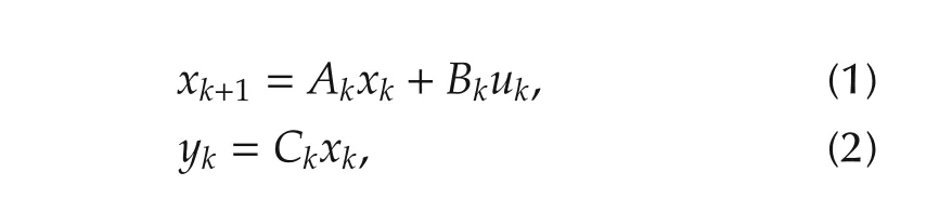
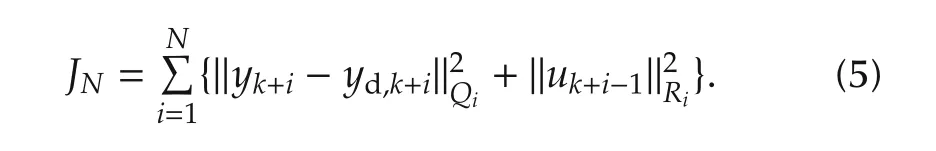
where xk∈Rn,uk∈Rm,and yk∈Rpare respectively the state,the input and the output at instant k.The matrices Ak,Bk,and Ckare of appropriate dimensions.It is assumed that the triplet{Ak,Bk,Ck}is known for all k.The goal of MPC or RHC in this paper is to seek a control law ukthat explicitly minimizes the performance measure

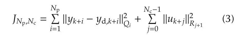
subject to the constraints(1)–(2).Here,Npand Ncare respectively the lengths of the prediction and control horizons,yd,kis the desired output of the system Σ at instant k,andand‖·‖Rjare quadratic norms,with Qiand Rjrespectively symmetric positive semi-definite and symmetric positive definite matrices:Qi≥0,1≤i≤Npand Rj＞ 0,1 ≤ j≤ Nc(By definition,for any X=XT≥0,where zTdenotes the transpose of z).This allows differential weightings over the horizons.Clearly,JNp,Ncis positive definite.Moreover,the measure(3)is merely the well-established finite-horizon linear quadratic tracking problem[34,35].The objective in(3)is to find over a finite horizon the required present and future control inputs uk,uk+1,...,uk+Nc−1that will minimize the tracking error over the finite horizon,where˜y≜y−yd.The matrices Qiand Rjachieve a trade-off between the two goals of minimizing the tracking-error energy and the required control energy.If we define the following quantities:

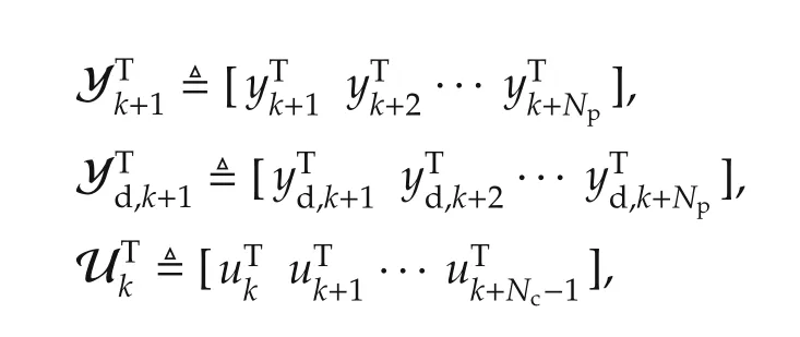
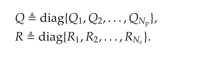
then(3)is equivalent to

where Q and R are defined as follows:

We note that in general the prediction horizon Npand the control horizon Ncsatisfy Nc≤Np.Indeed,the choice of Ncis often taken to be unity in industry.However,a smaller control horizon often leads to stronger and abrupt control action,and hence often referred to as aggressive control.Notwithstanding these considerations,the choice of Nc=Np≜N is quite typical in the literature.In that case,(3)is simply

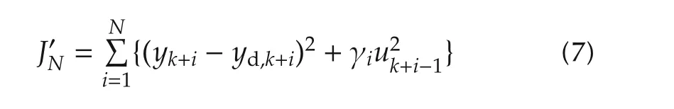
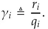
If all Qiand Rjin(3)are diagonal matrices so that Qi=diag{qi,1,qi,2,...,qi,p}and Rj=diag{rj,1,rj,2,...,rj,p},then the performance criterion(3)becomes

where yk+i,lis the lth component of the p-tuple yk+i,and so on.Clearly,it is possible to weight the individual inputs and outputs differently increasing the flexibility in the design.For single-input single-output(SISO)systems this further reduces to

2.1 The optimal solution

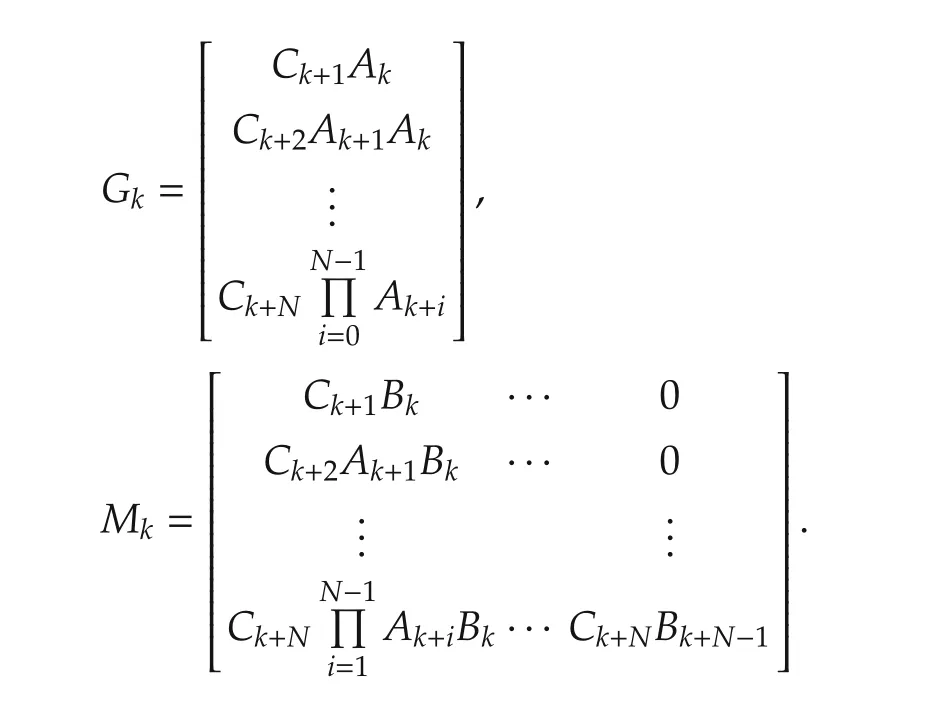
Given that the state-space representation(1)–(2)is known a priori,we first present the solution to the problem of finding the control input sequence that minimizes(5).Evidently,given the input sequence uk,uk+1,...,uk+N−1,we can predict at time instant k the outputs yk+1,yk+2,...,yk+Nfor any given finite horizon N;here,we have assumed that Np=Nc=N.Accordingly,we have the following relationship:

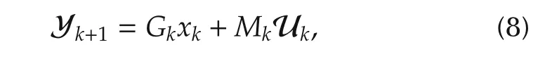
where Yk+1and Ukare as defined earlier,and Gkand Mkare respectively

If Σ is a linear time-invariant system Ak≡ A,Bk≡ B and Ck≡C;then the above matrices for the system with the state-space representation

are as follows:

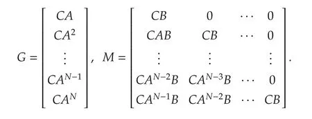
Clearly,G=Vo(C,A)A where Vo(C,A)is the extended observability matrix with N entries,and M is a lower triangular Toeplitz matrix of Markov parameters with Vo(C,A)B as the first column.

On setting the gradient of the performance criterion with respect to Uk(denoted∇UkJN)to zero,we obtain the control sequence that optimizes the objective function in(5):

CommentAn estimatecan be used if all the states are not measurable:

In contrast to other control techniques,the impact of MPC in industrial control problems is more significant largely due to its ability to handle simply and effectively hard constraints on the states and the control inputs;these are typically expressed as inequalities.In(3),the cost function JNp,Ncis convex as all its sub-level sets are ellipsoids.Each inequality constraint on the input corresponds to a half-space in Rm.We therefore define an admissible control space Ω in Rmwhich is the finite intersection of these half-spaces;evidently,Ω is convex.Similarly,the inequality constraints in the state space corresponds to a convex set χ in Rn(Constraints on the output can be translated as constraints on the state).Thus,MPC with the constraints(1)–(2)together with the hard constraints on the states and control input may be reformulated as the minimization of a convex function;this is nothing but a quadratic program(QP).We introduce the following definitions:

De finition 1Let χ and Ω be closed convex sets respectively in Rnand Rmsuch that the equilibrium state belongs to χ.We say that the pair(x,u)is admissible if for all time instants k,xk∈χ and uk∈Ω.

De finition 2A control strategy is said to be recursively feasible if,for any xk∈ χ,there exists a sequence{uk}∈Ω such that xk+1∈χ,∀k.

Let Ydbe the class of desired output trajectories such that for every yd∈Yd,there exists an admissible pair(x,u)such that yk≡yd,k.

De finition 3We say a given signal ydis trackable if and only if yd∈Yd,and u can be generated by some recursively feasible control law.

A characterization of sequences that are trackable by LTI systems is given in[38].

The constrained optimal control problem(5)can be formulated as a QP:

subject to the constraints(1)–(2).This can be solved using Hilderth quadratic programming(HQP)which is an interior point method.It is initialized with(11)and the dual variables are tuned iteratively while checking for constraint violations.The optimal value of the cost function can be reached without violating any constraints if sufficient number of iterations is allowed.

Since JNis positive definite the QP does not have multiple optima or unbounded solutions.If ydis trackable,then the solution is unique.Moreover,the solution lies either on the boundary or the interior of the feasible set.This solution approaches the standard linear quadratic tracking problem as N→∞.It is well-known that the LQR problem for(9)has a closed-form solution with the feedback gain a constant matrix that is used to determine the control inputOn the contrary,the QP(12)with N＜∞results in an optimal controlat instant k.MPC looks at an open-loop optimization problem that may lead to a larger variance in the tracking error in the future if left uncorrected.This can be averted by taking fresh measurements at every instant thereby allowing for corrective measures.Therefore,when measurements of the state are available at every instant,onlyfrom this sequence is applied at instant k,and other values discarded.If state measurements are not available at every instant,the computed future control inputs are used until the instant when the next measurement is made available[39,40].Evidently,such an approach has the advantage of a reduced overall computational complexity.

The choices of Npand Ncare crucial to ensure closed loop stability and recursive feasibility of the MPC algorithm.These parameters affect the size of the terminal set where the state xk+Nresulting fromexpected to lie.Larger terminal sets are preferred so that stability can be guaranteed for larger feasible sets.It is possible to enlarge the terminal set by increasing the values of the prediction and control horizons.However,there appearsto be anupper bound on Ncbeyondwhich the terminal set does not grow.In the next section we present a technique to determine an upper bound forNpbeyond which there is no significant improvement in the closed loop performance.Garriga and Soroush[41]provided a detailed study on the movement of the closed-loop poles with the changes in these parameters.

2.2 Prediction horizon and stability

A number of parameters affect the stability of the optimal control(11).Clarke et al.[9,10]discussed the effect of the design parameters Q,R,and N on the closed loop stability,performance,and computational efforts.The horizon N is perhaps the most important of these parameters as the computational complexity grows exponentially with N.It is perhaps impossible to devise a method that determines precisely its optimal value N∗,the smallest N for which the closed-loop system is stable.Nonetheless,offline techniques that provide an estimateofN∗have appeared in the past[16–20];clearly,ˆN∗≥N∗.However,these methods are computationally intensive and the resulting estimates conservative.

A technique to estimate an upper boundof N∗that guarantees closed-loop stability for controllable finitedimensional linear systems was proposed in[18].An important advantage of this method is that additional terminal constraints are not necessary to enforce stability.Indeed,for anythe following has been shown in[18].

Theorem 1Suppose that I is any compact set in the feasible region corresponding to(9).For any initial condition in I,there exists an upper boundso that the predictive control(11)for the regulation problem is stabilizing for any natural number.Further,JˆN∗is a Lyapunov function.

is a sub-level set in the feasible region of the state-space for some a priori chosen μ≤J∞.Clearly,forαN≤1+∈for some∈＞ 0,and αN→ 1 asThe estimated prediction windowˆN∗is the minimum value of N＞1 such thatWe note thatˆN∗not only results in a stabilizing MPC,but also ensures that the QP in(12)is recursively feasible.Moreover,the upper boundˆN∗determined by this method is conservative.Determining an upper bound that is less conservative is discussed in[21]and[42].

By posing as a couple of non-convex optimization problems,the quantities αNand σNcan be computed.There is however no guarantee on the global optimality[18].An alternative approach is as follows:Compute these quantities at every point in the sub-level set W.Since this is not quite practical,the set W is quantized to some desired resolution,and,for each choice of N,αNand σNcomputed at the grid points.Clearly,the computational complexity grows with the size of W,the desired resolution,and N.Accordingly,this procedure is not readily scalable to higher order systems.

Our interest in this paper is more than the problem of regulation.Even in the case of tracking a fixed set-pointan MPC with a fixed horizonrequires a reference governor after introducing a change of variables x−¯x andwhere each trackable fixed set-point corresponds to a steady-state admissible pair(¯x,¯u).Once this pair is computed,the set-point tracking problem canbe formulated as a QP.However,the MPC formulation(12)with performance measure(5)is designed to handle explicitly the more general tracking problem without such a change in variables.We emphasize that for the tracking problem,a single value forobtained by the procedure in[18]is perhaps not suitable as it targets only state-regulation and may not guarantee good tracking performance.Moreover,such a choice ofmay fall short in addressing robustness issues.Accordingly,unreasonable offline computational efforts to computeis not justified for systems with modelling uncertainties,or for those systems that are expected to track arbitrary references.On the contrary,in this paper we consider dynamically varying the prediction horizon.This avoids the need to recomputefor every change in the reference,and is an aid to make MPC robust.

2.3 MPC based on multiple-controllers and switching

Tracking a priori chosen signals yd∈Ydis the goal in this paper.As mentioned earlier,determiningis not justified.We present here a technique that uses switching to automatically and dynamically choose an appropriate value of the prediction horizon at each instant k.This results in a time-varying horizon.Given system(9)–(10),there exists some N∗that is stabilizing.Using the procedure in[18],it is possible to arrive at a conservative estimateMoreover,by Theorem 1,anyis stabilizing.Thus,in our approach,we merely choose a sufficiently large prediction horizon.This naturally reduces the design overhead of explicitly computingpriori.The overall scheme is depicted in Fig.1.Here,K isa bank of N controllers Cw,1≤w≤N,alloperating in parallel.All of these controllers adopt the receding horizon policy and solves the QP(12)with the prediction window w in(5).Of these N control inputs,we choose the one that minimizes the performance measure(13).This decision block is represented as D in Fig.1.We have the following result.

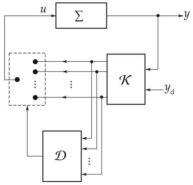
Fig.1 MPC with time-varying horizon.

Theorem 2Consider system(9)–(10).Let at each instant k,

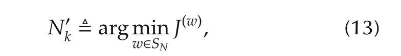
Here,ydis any trackable output,y(w)is the output of(9)with u(w)as the input,and u(w)is the solution to QP(12)with N=w.Then,the receding-horizon control with the sequence of prediction windowsis both recursively feasible and stabilizing.Moreover,the resulting control action results in a lower cost compared to minimizing(5)with fixed prediction horizon.

ProofWithout loss of generality,letandEvidently,N sufficiently large implies that N∗≤.By Theorem 1,a receding horizon policy with any N ≥N∗is stabilizing.Moreover,JNis a Lyapunov function;therefore,JN(k+1)＜ JN(k),∀k.Further,by construction,Ji(k)≤ JN(k),∀i≤ N and∀k.For any k,and N′≤ N.Accordingly,

clearly preserving the monotonicity.Therefore,JNcontinues to be the Lyapunov function and stability of the closed loop is guaranteed with the proposed MPC with time-varying prediction horizon.Moreover,whenever,the RH controller with prediction horizon w places the pair(xk+1,uk+1)closer to the steady-state value(¯x,¯u)than any other RH controller in K,proving that tracking performance is improved with switching.

Commentsi)The matricesandmay be chosen independent of Q and R in(5).When required,this flexibility may help in improving the overall performance.ii)The structure of Fig.1 was used in[23]to demonstrate the improvement in performance in the context of state-regulation,and in[25]for tracking a set-point.

2.4 MPC with multiple models for robustness

The MPC solution(11)is a sequence of future control inputs resulting from an open-loop optimization procedure.It has been observed in[43]that an open-loop MPC solution cannot guarantee good approximation to the globally optimal solution in the presence of modelling uncertainties.However,a time-varying control law involving open-loop MPC procedure may be adequate for a linear system with quadratic cost[43].The framework presented in Section 2.3 results in a time-varying MPC control.This can be adapted to introduce robustness to modelling uncertainties.

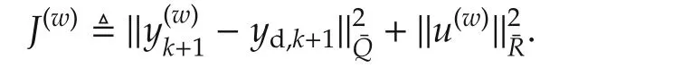
In this paper,we restrict our attention to modelling uncertainty of the parametric type.Let Anom,Bnomand Cnombe respectively the nominal system,input and output matrices of the given plant.We assume that the true model lie in known sets that are described as follows:

where the real constants αi,1 ≤ i≤ 6 are such that α1＜α2,α3＜ α4,α5＜ α6,and the triplet{Anom,Bnom,Cnom}corresponds to the nominal state-space representation(9)–(10).

We choose a sufficient number of models that are representative of such uncertainties;that is,we choose a sufficient but finite number of α in the corresponding intervals.For each model we choose an upper bound on the prediction horizonˆN∗and obtain a set of control laws as described in Section 2.3.

Evidently,the decision block D represented by(13)chooses that control law with the minimal one-step ahead cost.Suppose that the overall scheme switches to a particular model at instant k and uses this model for all subsequent instants.Then,according to Theorem 2,the control action results in.Moreover,the sequence of control inputs results in a monotonically lower cost compared to minimizing(5)with fixed prediction horizon.On the contrary,if it switches to a different model,the corresponding cost is lower by virtue of the fact that it was chosen by minimizing the one-step ahead cost(13)with the expectation that the state of the plant is driven closer to the desired state.There is,however,no guarantee of monotonicity.From the simulation results presented in Section 3 we demonstrate that multiple models can make MPC robust to such modelling uncertainties.

3 Simulation results

In this section,we demonstrate the advantages of using a time-varying horizon and multiple models for the problems of i)regulation,ii)tracking varying set-points,and iii)tracking a class of reference trajectories.We illustrate using the following examples:

·System I:a stable system.

·Systems II and III:unstable systems.

·System IV:the Shell heavy oil fractionator benchmark problem.

·System V:a servomechanism.

·System VI:a time-varying system.

In what follows,we compare the performance of conventional MPC(Method A)with that of an MPC with time-varying horizon(Method B)and an MPC with multiple models and time-varying horizon(Method C).These methods are often respectively referred to as MA,MB,and MC.

3.1 System I:a stable system

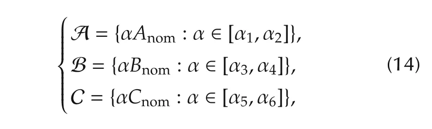
The dynamics of a stable second-order LTI system consideredin[18]istakenfrom[44],hasthestate-space description

and is referred to as System I in the sequel.Using the procedure outlined earlier in Section 2.2,an estimate of the optimal prediction horizon for this system isFollowing[18],the input to the system is constrained by the inequality|uk|≤0.5 for all k,and the initial condition is assumed to lie in the following region in the state-space:

We illustrate the application of this prediction win-dowfor both regulation and tracking of an arbitrary signal.For the tracking problem,we consider the output variable of interest as the first state of(15).Three scenarios are considered for simulations:i)Scenario 1:regulation without modelling uncertainty or exogenous inputs;ii)Scenario 2:regulation with exogenous inputs and without modelling uncertainty,and iii)Scenario 3:tracking in the presence of modelling uncertainty.

ForScenarios1and2,weconsider thenon-zeroinitial condition:and for Scenario 3,we assume the initial state to be the origin.The exogenous inputs for Scenario 2 appear in the form of a disturbance at the input and measurement noise,both of which are 1 dBW white Gaussian noise signals.To deal with modelling uncertainty in Scenario 3,we use three models whose system matrices respectively are A(Model 1),0.8A(Model 2),and 1.2A(Model 3),where A is the system matrix in(15).Sincefor System I and we consider three models for Method C,there are a total of 15 controllers in the block K of Fig.1;of these,the first five controllers correspond to the nominal Model 1(numbered 1 through 5),the next five to Model 2(numbered 6 through 10),and the last five to Model 3(numbered 11 through 15).

The simulation results for System I for all scenarios are shown in Figs.2–7.The evolution of the states x1and x2for Scenario 1 are compared in Fig.2 using all the three methods.Clearly,the performance of all methods appears to be rather similar in that the peak values and the settling times are approximately the same for all methods.Accordingly,it is expected that the control inputs for the three methods are similar.Indeed,it is evident from Fig.3(a)that only Method C requires a control input that is marginally different.The switching histories between the different control laws are shown in Fig.3(b)for both Methods B(indicated by circles)and C(indicated by diamonds).Evidently,in an ideal situation like Scenario 1,we observe that there is very little advantage of using either Method B or C.In fact,with Method B,there is only a 0.13%improvement for a 3.18%increment in the control energy when compared to conventional MPC.On the contrary,it is obvious from Fig.3(b)that the switching strategy has chosen the second model(Model 2)whose dynamics differ from the nominal to an extent of 20%.Consequently,both tracking-error and control energies with Method C are higher than those obtained with either Methods A or B.The tracking-error and control energies for Scenario 1 are tabulated in Table 1.These values indicate that Method B performs marginally better than Method A in the sense of lesser tracking-error energy but at the cost of a slightly increased input energy.With the particular choice of models and switching criterion,Method C favoured the decrease in the control energy at the cost of a marginal increase in the energy in the tracking-error.

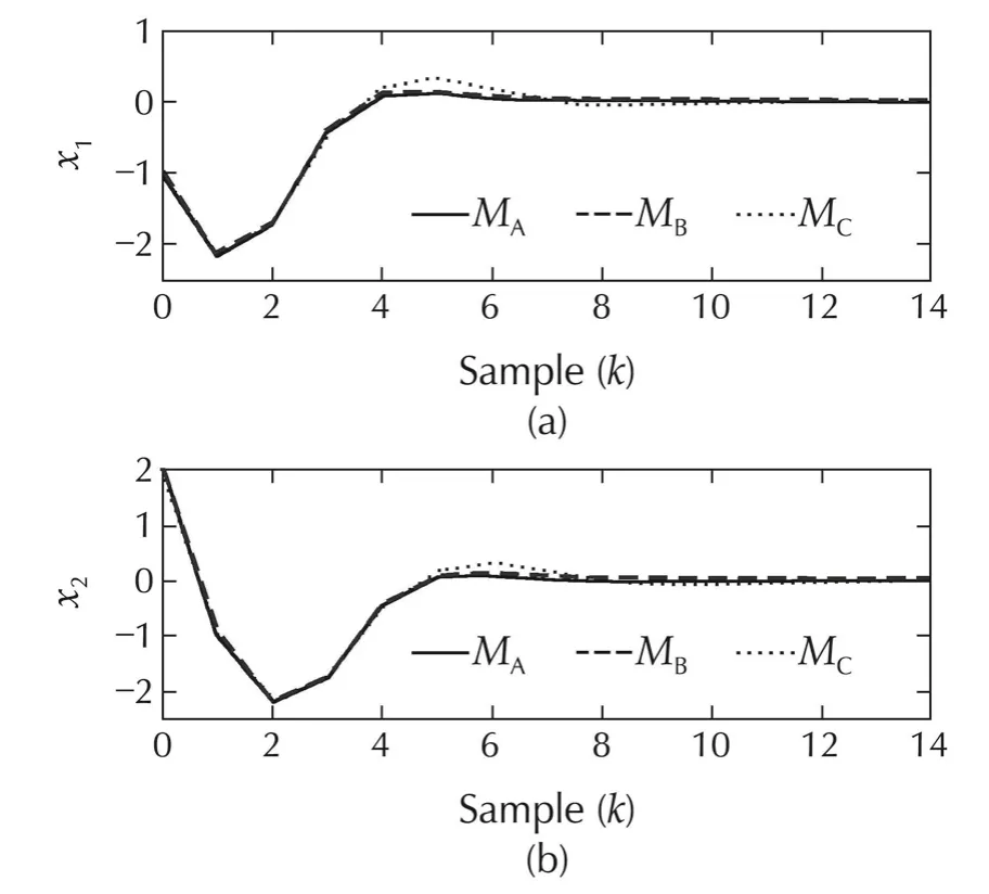
Fig.2 Scenario 1 of System I:comparison of regulation performance with conventional MPC(Method A:MA)with that of MPC with time-varying horizon(Method B:MB)and MPC with multiple-models and time-varying horizon(Method C:MC).(a)State x1.(b)State x2.

Fig.3 Scenario 1 of System I.(a)Input signals required for MethodsA,B and C.(b)Switching histories for Methods Band C.

The performance of the three approaches in the presence of exogenous inputs and no modelling uncertainties(Scenario 2)is similar to that of Scenario 1.As shown in Fig.4,the evolution of the states is similar for all methods indicating that the regulation performance in the presence of the chosen exogenous inputs of all methods is comparable.Moreover,when Fig.5(a)is compared to Fig.3(a),it is evident that the inputs required for Scenario 2 are also similar to that of Scenario 1.Similar to Scenario 1,Method C has again chosen the second model.The tracking-error and control energies for Scenario 2 are tabulated in Table 1.Again,these values indicate that Method B performs marginally better than Method A in the sense of lesser tracking-error energy but at the cost of a slightly increased input energy.With the particular choice of models and switching criterion,Method C has again favoured a decrease in the control energy at the cost of a marginal increase in the energy in the tracking-error.

Fig.4 Scenario 2 of System I:comparison of regulation performance with Methods A,B and C.(a)State x1.(b)State x2.

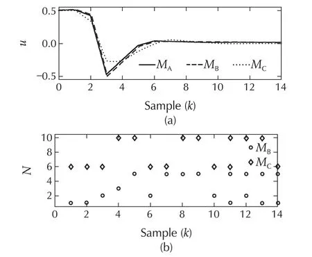
Fig.5 Scenario 2 of System I.(a)Input signals required for Methods A,B and C.(b)Switching histories for Methods B and C.

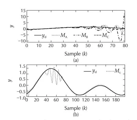
Fig.6 Scenario 3 of System I:comparison of tracking performance.(a)Methods A,B and C.(b)Method C.

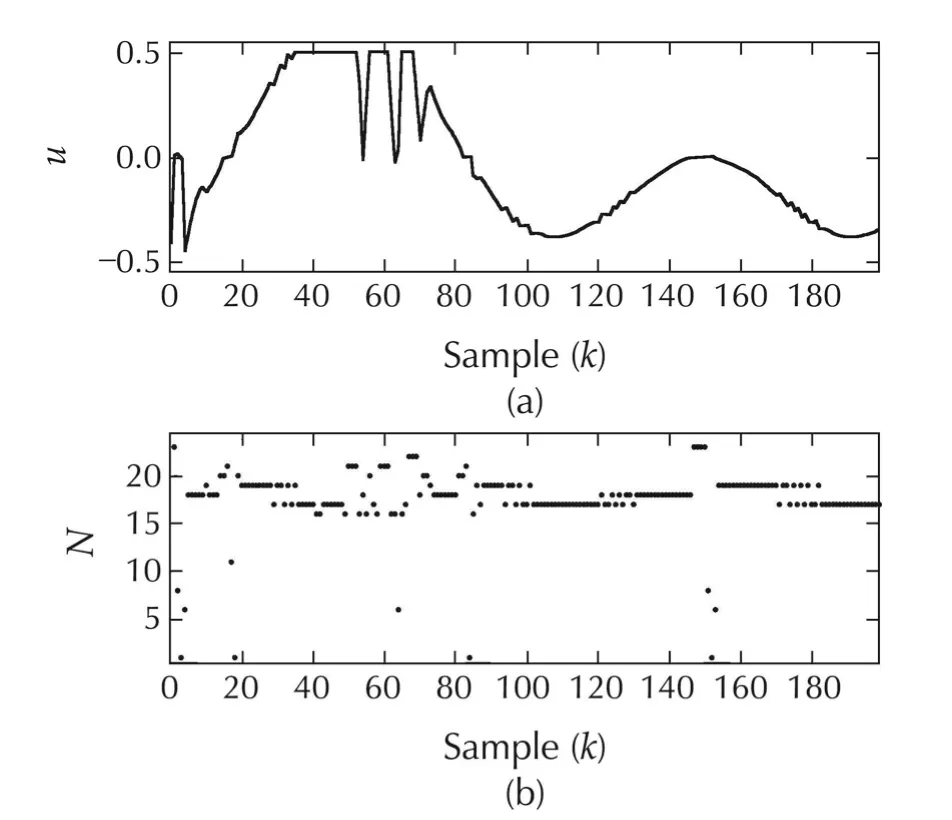
Fig.7 Scenario 3 of System I.(a)Input profile with Method C.(b)Switching history for Method C.

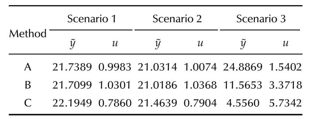
Table 1 System I:comparison of performance.

In contrast to Scenario 1 and Scenario 2,the performance of MPC with multiple models and time-varying horizon(Method C)is far superior in the presence of modelling uncertainties.This is evident from Fig.6.Indeed,both Method A and Method B are unable to stabilize the system and ensure that the output track the desired trajectory.This is primarily due to the hard constraint on the input which causes insufficient control action to bring the states to the required regions in the state-space.However,with multiple models,the control action is sufficient despite the hard constraints.The tracking performance is certainly poor in the time range 40≤k≤70.This can again be attributed to the hard input constraints as is evident from Fig.7(a).Nonetheless the overall system recovers with perceptibly no tracking errors beyond k=80.

3.2 Systems II and III:unstable systems

System II is the example unstable system considered in[18].Its state space description is as follows:

An estimate of the optimal prediction horizon for this system isfor the state-regulation problem[18].The sub-level set in the feasible region χ ={x ∈ R2:|Cx|≤ 2}is chosen to be W={x∈ R2:|x1|≤ 0.5,|x2|≤0.5}.Clearly,W is in the interior of χ.This set is quantized with a resolution of 0.1 resulting in 100 distinct points.The quantities αNand σN,defined in Section 2.2,are computed for different values of N＞1.We note that if the resolution is improved to 0.01 these computations are to be carried out for10,000points.It is quite obvious that there is an exponential growth in the offline computational effort if better estimates of N∗are required.Moreover,the objective here is that the output of System II tracks a varying set-point.This implies that N∗is to be determined for each such set-point.However,as mentioned earlier,we avoid such computations by merely choosing a sufficiently high value of N.

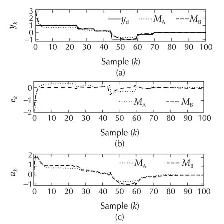
Fig.8 System II with using Methods A and B.(a)Output responses.(b)Tracking errors.(c)Input signals.

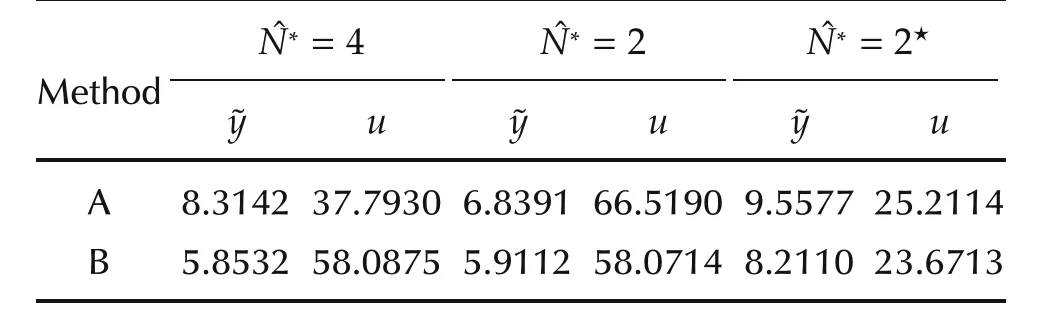
Table 2 System II:comparison of Methods A and B.

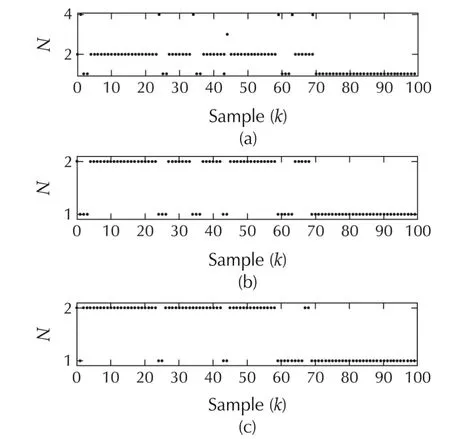
Fig.9 Switching histories for System II.(a)WithˆN∗=4.(b)WithˆN∗=2.(c)With 20%uncertainty andˆN∗=2.

Although the proposed strategy to address robustness issues in this paper is Method C,we now show that Method B can be used to address parametric uncertainty in this example system.Assuming a 20%parametric uncertainty,the results of the simulation experiment with ˆN∗=2 are shown in Fig.11,and tabulated in Table 2(c).We again observe a similar trend:The performance of an MPC with time-varying horizon is better than conventional MPC,with a reduction of 14.09%in the tracking error energy.A comparison between Table 2 shows that the control effort required for this experiment is lesser in the latter case despite the uncertainty.This is due to the fact that the parametric change in the system matrix for this example ensures that the poles move closer to the origin.

Clearly,with this example it appears that MPC with time-varying horizon is able to handle the class of modelling uncertainties considered in this paper.However,as demonstrated earlier for System I,this method may not always guarantee robustness.Multiple models are required to ensure this.

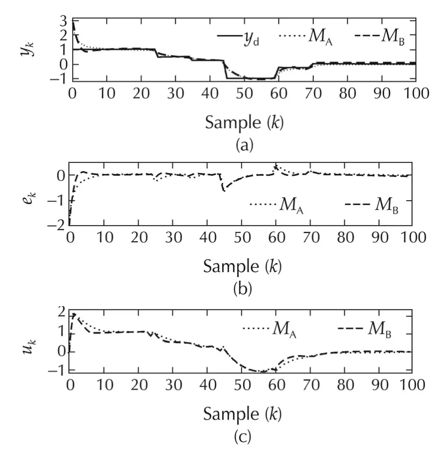
Fig.10 System II with using Methods A and B.(a)Output responses.(b)Tracking errors.(c)Input signals.

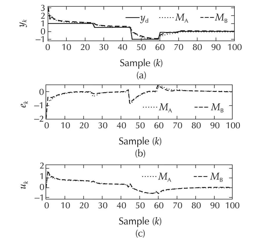
Fig.11System II with 20%uncertainty and using Methods A and B.(a)Output responses.(b)Tracking errors.(c)Input signals.

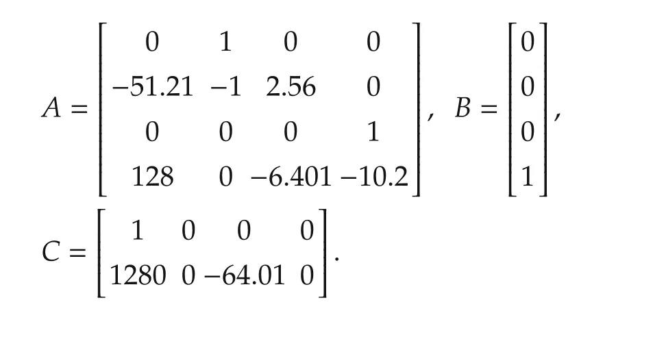
The second unstable example(System III)that we consider has the state-space description

The system dynamics is clearly unstable.For this example we consider the problems of regulation with modelling uncertainties,and tracking an arbitrary reference signal in the presence of modelling uncertainties.The desired output signal for this system is chosen to be

The application of the procedure in[18]to determine an optimal value N∗of the prediction window is not straightforward.For unstable systems,the prediction horizons ought to be chosen with sufficient care.For this example,it has been the experience that the tracking performances with conventional MPC(Method A)for N≥10 are quite similar.Thus,in this paper we chooseto be 10 for conventional MPC.For Methods B and C the presence of switching can lead to rather undesirable results.Experience indicates that the choices of 8,9 and 10 for the prediction-horizon yield the best results.We use five models for MPC with multiple models and time-varying horizon.The system matrices for these five models are 0.8A,0.9A,A,1.1A,and 1.2A respectively.Thus,the controller block K in Fig.1 has 3 control laws for Method B and 15 control laws for Method C.The regulation problem is simulated with the initial condition[1 1]Tand the tracking problem is simulated with as[0 0]T.A modelling uncertainty of 50%is assumed for both simulation cases;i.e.,the actual system matrix is assumed to be 0.5A.

The simulation results for System III are presented in Figs.12–15.A comparison of the regulation performances shown in Fig.12 shows that MPC with multiple models and time-varying horizon(Method C)performs better than the other methods;a reduction of 51.74%in the tracking-error energyis observed.The performances of conventional MPC and MPC with time-varying horizon are comparable.Interestingly,the control energy is reduced by 59.21%with Method C.Even though the states converge to the origin at the fourth time instant for all three control techniques,they move closer to the origin faster with Method C.The control inputs for the three strategies are depicted in Fig.13(a).The switch with ing histories for Methods B and C are shown in Fig.13(b).It can be observed that only two models are used in Method C.The error and control energies are tabulated in Table 3.

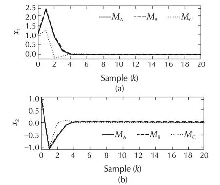
Fig.12 System III:comparison of regulation performance with Methods A,B and C.(a)State x1.(b)State x2.

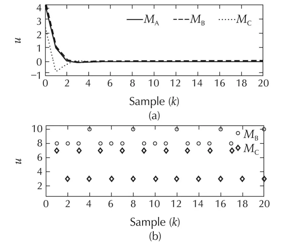
Fig.13 System III.(a)Input signals for Methods A,B and C.(b)Switching histories for Methods B and C.

The tracking performances of the three methods for System III are shown in Figs.14 and 15,and the results summarized in Table 3.It is again observed that the performance with Method Cis considerably better than that of the performance with Methods A and B.There is a reduction of 50%in the tracking-error energy,but with a considerable increase in the control energy.On the contrary,the performance of the Methods A and B are comparable.In the presence of modelling uncertainty,Method C is therefore found to perform better.

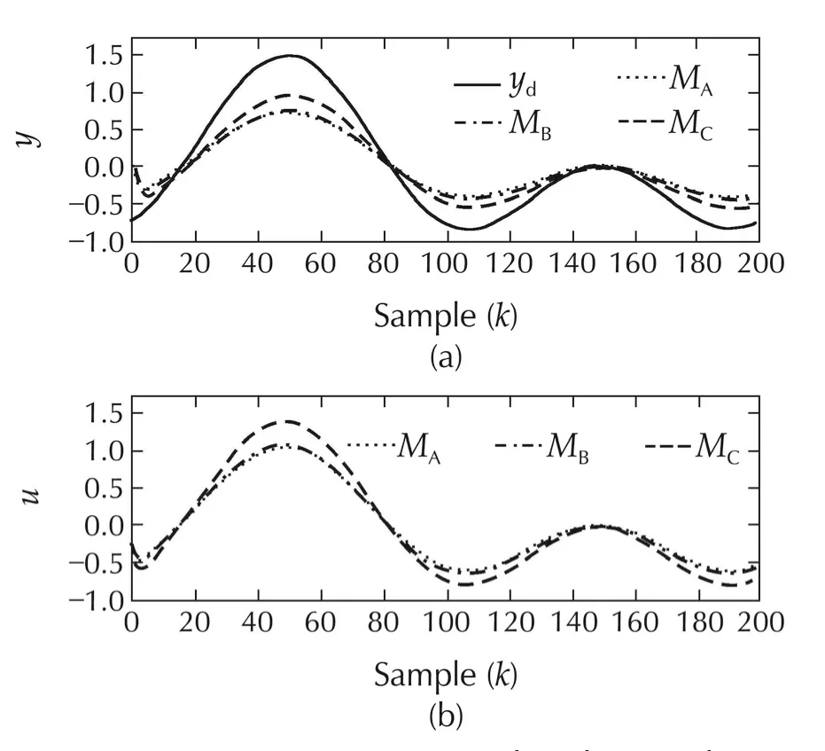
Fig.14 System III.(a)Comparison of tracking performance with Methods A,B and C.(b)Input profiles for the three methods.

Fig.15 System III:switching histories.(a)Method B.(b)Method C.

Table 3 System III:comparison of performance.

3.3 System IV:the Shell heavy oil fractionator benchmark problem

The Shell heavy oil fractionator is a highly-constrained multivariable non-square process with large dead times.The problem of regulating this system about a nominal point was proposed by Prett and Morari in 1987[45],and as a benchmark problem by IFAC[46].The steadystate values of the controlled variables,the magnitudes of modified variables and their delta-changes from time to time are constrained.We consider a square sub-part of the presented model with three product draws and three side heat circulating loops.The three output variables of interest are the top end point(TEP),the side end point(SEP)and the bottom reflux temperature(BRT).The control inputs are the top draw(TD),the side draw(SD)and the bottom reflux duty(BRD).The unmodelled disturbances are the intermediate reflux duty(IRD)and the upper reflux duty(URD).

The transfer function matrix for the three-input threeoutput system is given by

where y1,y2and y3respectively are TEP,SEP and BRT,and u1,u2and u3respectively are TD,SD,and BRD.The effect of the disturbances on the three outputs is modelled as follows:

where d1and d2are respectively IRD and URD,the unmodelled disturbances.All the entries Gij(s)and Hij(s)in these transfer function matrices are modelled as firstorder systems with dead-time[46]:

where the units of θ and τ are in minutes.The values of the parameters K,θ and τ are given in Table 4(a)with the uncertainties in the gains of the model in Table 4(b),where−1≤ ∈i≤ 1,1≤ i≤ 5.

The specifications for the top and side draws are determined by economics and operating requirements.There is no specification for the bottom draw.The three loops remove heat to achieve a desired product separation.The energy acquired by the heat exchangers is used to reheat other parts of the overall process;accordingly,the heat-duty requirements are time-varying.

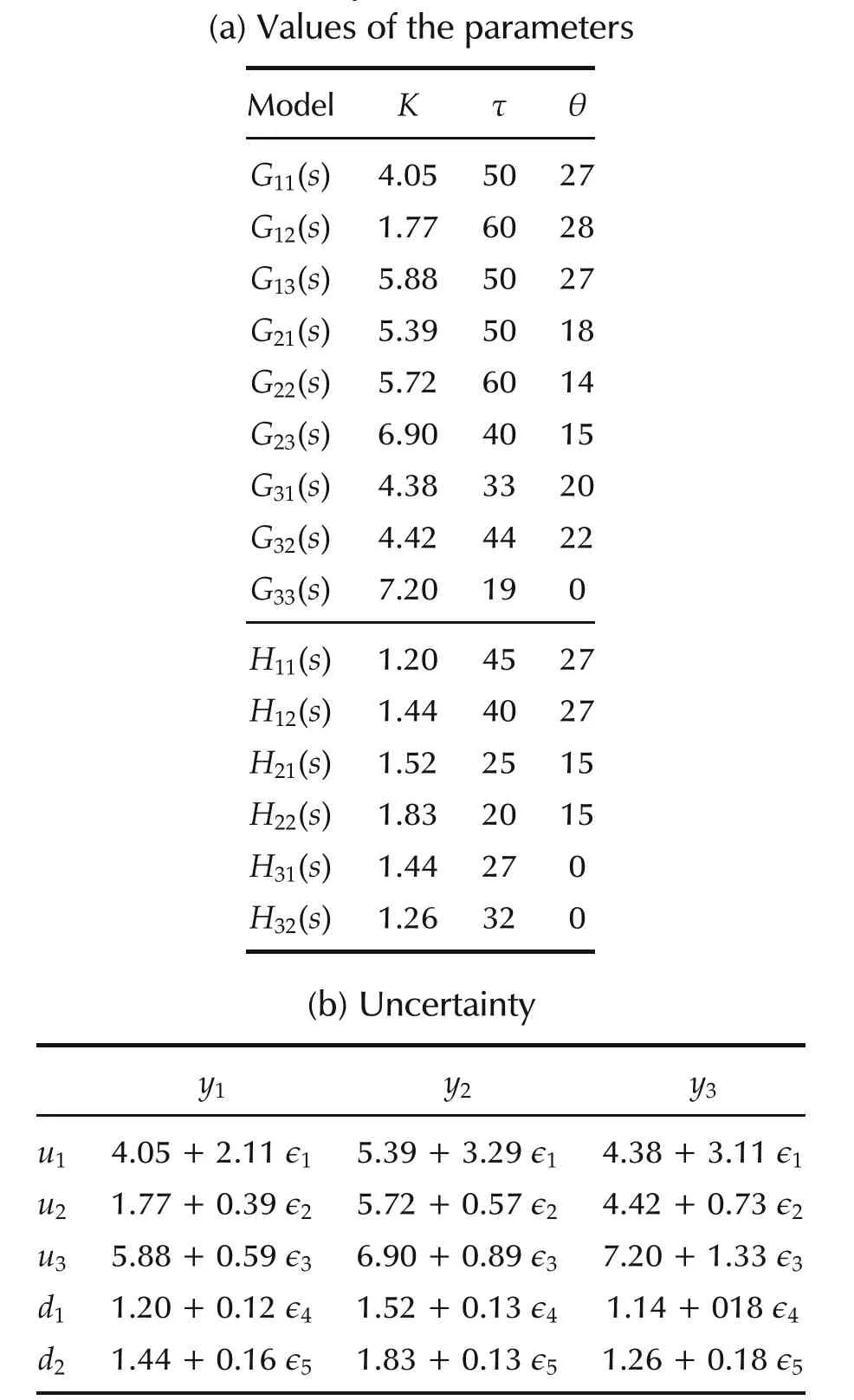
Table 4 Parameter values and uncertainty for the Shell problem.

Using a fifth-order Pad´e approximation for the delays,the continuous-time model is discretized with a sampling interval of 1 minute.The dimension of the resulting discrete-time state-space model is 100.Naturally,computingˆN∗for this system as discussed in Section 2 is a formidable task.However,a choice ofˆN∗=5 is found to be sufficient to ensure good performance for the regulation problem.We consider here a changing set-point for SEP even though the original objective is regulation.The set-point is chosen in a manner so that it does not violate any constraints specified in[46]subject to the requirements that there are no deviations from the constraints imposed on other variables.The following five test cases are considered for simulations in this paper[46]:

1)Case 1:∈1= ∈2= ∈3= ∈4= ∈5=0;URD=0.5;and IRD=0.5.

2)Case 2: ∈1= ∈2= ∈3= −1,∈4= ∈5=1;URD=−0.5;and IRD=−0.5.

3)Case 3:∈1= ∈2= ∈3= ∈4=1,∈5= −1;URD=−0.5;and IRD=−0.5.

4)Case 4:∈1= ∈2= ∈3= ∈4= ∈5=1;URD=0.5;and IRD=−0.5.

5)Case 5:∈1= −1,∈2=1,∈3= ∈4= ∈5=0;URD=−0.5;and IRD=−0.5.

Of these prototype test cases,we present the results only for Cases 1 and 3:Case 1 considers addition of the two specified constant disturbances and introduces no modelling uncertainty.Case 3 is closer to the practical scenario where modelling uncertainties and disturbances are present.Although this is a benchmark problem for regulation,we consider here the situation wherein the variable SEP track a varying set-point.

We compare the output variable of interest(SEP)with the desired set-point for Case 1 in Fig.16.The results with conventional MPC(Method A)and with time-varying horizon MPC(Method B)are respectively shown in Fig.16(a)and(b).As observed earlier in the previous examples,we see an improvement in the tracking performance with Method B when compared to conventional MPC.There are no violations of any other imposed constraints.The tracking-error energy reduces from6.1144to 5.6686.The variables TEP and BRT and the three inputs TD,SD and BRD are compared in Fig.17 for Methods A and B.The switching history is also shown.

Fig.16 System IV:comparison of desired SEP and actual SEP for Case 1.(a)Method A.(b)Method B.

Similarly,the desired and actual outputs for Case 3 with Method A are shown in Fig.18(a)and with Method B are shown in Fig.18(b).The tracking-error energy re-duces from 9.4389 to 8.5641.The profiles of TEP,BRT,the three inputs for this case are depicted in Fig.19;and this also includes the switching history.It is evident from the switching histories for both cases that the horizon N=5 is chosen only for the first few minutes when there are larger transients;and subsequently,it chooses N=1.

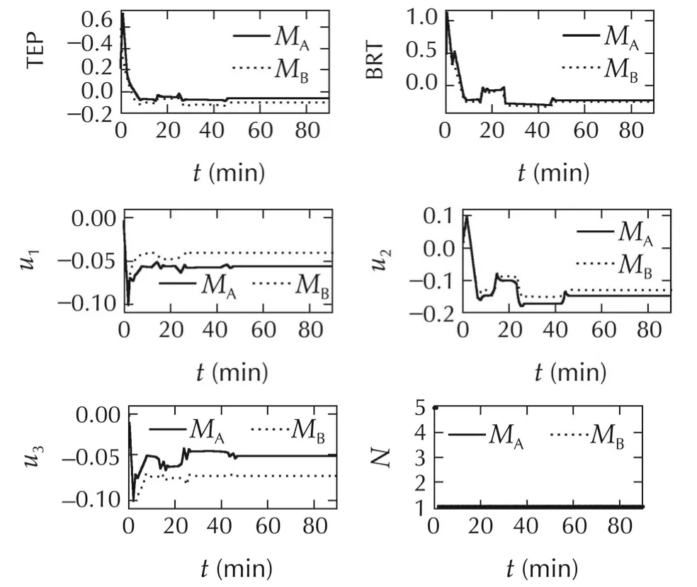
Fig.17 System IV:the variables TEP and BRT,and the three inputs TD,SD and BRD for Case 1.The switching history with Method B is also shown.

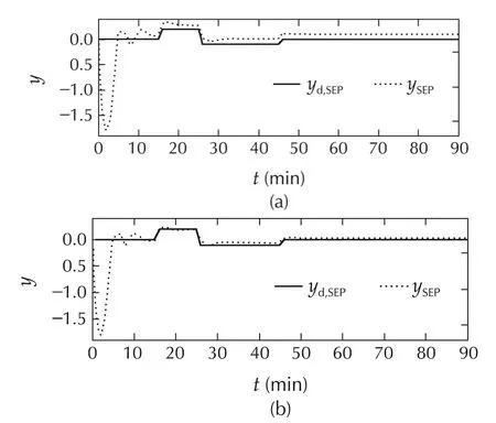
Fig.18 System IV:Comparison of desired SEP and actual SEP for Case 3.(a)Method A.(b)Method B.

Moreover,in the presence of uncertainty and disturbances,the response with Method B settles down faster and with lesser tracking error.The tracking-error energies in the period from 10 minutes to 90 minutes with MethodBare0.14and0.20asopposed to0.19and0.97 withMethodAforCases1and3,respectively.Evidently,for this benchmark problem,MPC with time-varying MPC is sufficient to make the overall system more robust to the considered disturbances and modelling uncertainties.Accordingly,the results with Method C(MPC with multiple models and time-varying horizon)are not presented.We emphasize that computingˆN∗for this 100th order system is rather difficult.On the contrary,in our approach we merely choose a sufficiently high upper bound.Moreover,MPC is made more robust by allowing the possibility of choosing an appropriate prediction horizon at every instant.

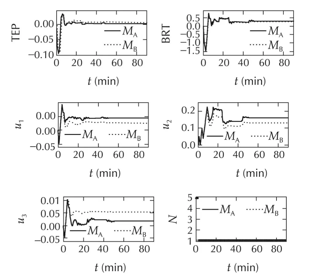
Fig.19 System IV:The variables TEP and BRT,and the three inputs TD,SD,and BRD for Case 3.The switching history with Method B is also shown.

3.4 System V:a servomechanism

The servomechanism considered here consists of a DC motor,a gear-box,an elastic shaft and an uncertain load[47].The fourth order state space representation of this system is as follows:

where

If θLand θMare respectively the load and motor angles,the state-vector of the system isThe outputs of interest are the load angle y1and the motor torque y2.The input to the system is a voltage signal whose value is constrained to lie within the range[−220,220].The objective is to maintain the load angle y1at a desired position.In addition,the torque is to satisfy the inequality|y2|≤ 78.5N·m.The system is discretized with a sampling interval of 0.1s with a zero-order hold on the input voltage[47].

As per the procedure outlined earlier in Section 2.2,the best estimate of the optimal prediction horizon for this case has been computed in[24]to beˆN∗=12.Tracking time-varying set-points was treated in[24].It was shown that the tracking performance considerably improved.Moreover,the overshoot and steady-state error reduced.This was achieved with only control laws corresponding to N=12 and N=1.In this paper,we study the effect of modelling uncertainty.It is assumed that there is a 50%modelling uncertainty in the system dynamics,i.e.,the actual system is described by the pair(0.5A,B).The goal in this paper is to tracka time-varying reference for the load angle without violating any of the hard constraints.For Method C,we used seven models.

The output responses of the system with the three methods are shown in Fig.20.The desired output is also shown.

Fig.20 System V:comparison of tracking performance.(a)Method A.(b)Method B.(c)Method C.(d)Torque for all methods.

Evidently,all the methods eventually settle down and track the desired trajectory.However,Method C outperforms the other methods.As is evident from Table5 the tracking-error energy reduced by 41.2%and this has been achieved with lesser control energy.Moreover,no constraints have been violated.This is evident from Fig.20(d)and Fig.21 that shows the respective profiles of the torque and the input signals.The switching history is shown in Fig.21(d).

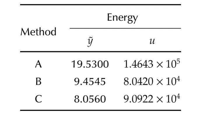
Table 5 System V:comparison of performance.

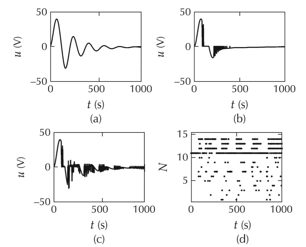
Fig.21 System V:input profiles for(a)Method A.(b)Method B.(c)Method C.(d)Switching history for Method C.

3.5 System VI:a time-varying system

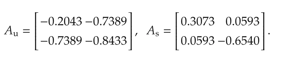
In this section,we present the simulation results of the proposed technique to a class of systems that changes its dynamicsin real-time.Such changesmay occur if,for example,there is a fault.In whatfollows,weconsider an artificial system whose dynamics change in a manner so that the system matrix switches from an unstable matrix Auto a stable matrix As:

The output and input matrices are as follows:

Thus,the system is described by the state-space de-scription:

where Akswitches from Auto As,and it is assumed that this takes place at k=50.The objective is that the output of System VI track a set-point of unity magnitude until k=50,and subsequently track a set-point of magnitude 0.5.To this extent,it is assumed that the precise instant of change in the dynamics is known.As initially discussed in Section 2,MPC can be applied to linear time-varying systems,and the finite-horizon optimal controller for such systems developed there.Further,we allow for a time-varying cost function where Q1=1,R1=0.1 for k≤50,corresponding to Au,and Q2=1,R2=0.5 for k＞50 corresponding to As.Thus,in this example,the system dynamics,the performance criterion,and the desired set-point change with time.From experience we use a horizon N=5 for all three control strategies.We use 10 models for Method C where the system matrices are scaled by factors of 1.4,1.25,1.0,0.75,and 0.6.Thus,there are 5 control laws in the block K in Fig.1 for Method B,and 25 control laws for Method C.

The results of the simulation experiments are depicted in Figs.22–25 and summarized in Table 6.The tracking errors for the three control strategies are shown in Fig.22.We observe that there is a significant decreasein the tracking-error energy with Method B.In fact Method B results in 81.86%reduction in the tracking-error energy with a mere 5.02%increase in the control energy relative to conventional MPC.The performance of both Methods B and C are comparable,with the latter yielding as lightly higher tracking-error energy but with much lesser control effort(We note that the weighting matrices determine this choice).However,the peak-to-peak variation with Method B is much higher when compared to that obtained with Method C.The input signals for the three methods are shown in Fig.22(a),with the switching histories for Methods B and C respectively in Fig.22(b)and(c).

In Figs.24 and 25,we present the simulation results under similar conditions as before with the following change:we assume a 50%uncertainty in the system matrix.We observe that Method B provides a 51.67%reduction in the control energy when compared to that with conventional MPC while spending 6.09%control energy in excess.This trend is similar to the earlier case.However,unlike the earlier case,Method C outperforms the other two control strategies in the presence of modelling uncertainty.The tracking error energy with Method C is 80.6%lesser than that with Method A and 59.87%lesser than that with Method B.The control energy too sees a 29.49%reduction compared to Method A and a 33.54%reduction compared to Method B.Similar to all the examples considered earlier,MPC with multiple models and time-varying horizon appears to be essential for handling modelling uncertainties.

Fig.22 System VI:tracking performance with the three methods.(a)Method A.(b)Method B.(c)Method C.

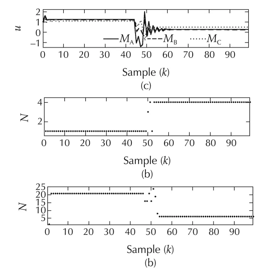
Fig.23 System VI.(a)Input signals for the three methods.(b)Switching history for Method B.(c)Switching history for Method C.

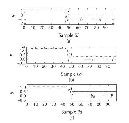
Fig.24 System VI with modelling uncertainty:tracking performance with the three methods.(a)Method A.(b)Method B.(c)Method C.

Fig.25 System VI with modelling uncertainty.(a)Input signals for the three methods.(b)Switching history for Method B.(c)Switching history for Method C.

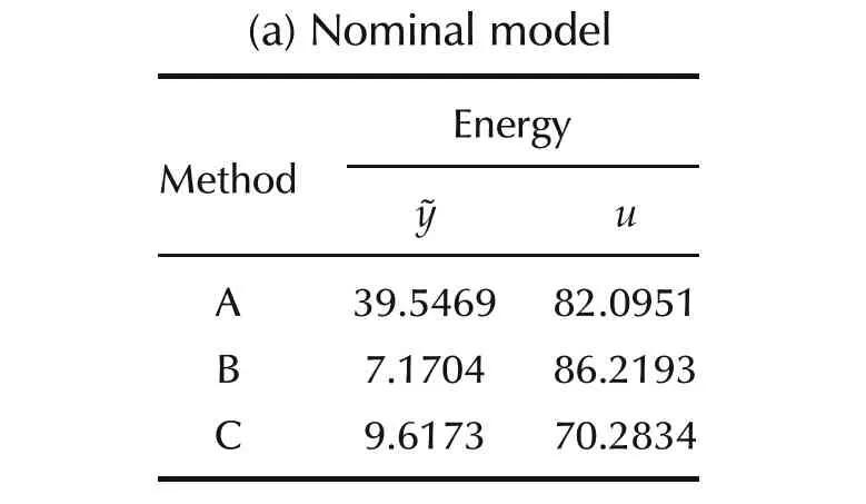
Table 6 System VI:comparison of performance.

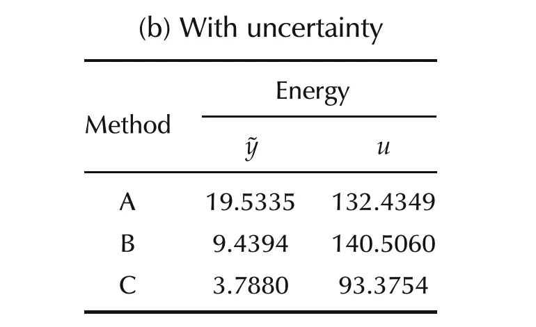
(b)With uncertainty Energy Method˜yu A 19.5335 132.4349 B 9.4394 140.5060 C 3.7880 93.3754

4 Conclusions

A method to not only optimally choose at every instant the prediction horizon in a receding-horizon type control but as well handle modelling uncertainties is proposed in this paper.Whilst the former is achieved by switching between multiple controllers designed using the receding horizon policy,the latter is achieved by introducing multiple models,and designing additional similar control laws.The stability of the overall system is discussed.The simulation experiments show a considerable improvement in the tracking performance.Whilst for some situations,only the time-varying horizon is sufficient to provide better performance,it is observed multiple models provide stability and improved performance in the presence of modelling uncertainties.

[1]A.I.Propoi.Use of linear programming methods for synthesizing sampled-data automatic systems.Automation and Remote Control,1963,24(7):837–844.

[2]M.D.Rafal,W.F.Stevens.Discrete dynamic optimization applied to on-line optimal control.AIChE Journal,1968,14(1):85–91.

[3]J.Richalet,A.Rault,J.L.Testud,et al.Model predictive heuristic control:applications to industrial processes.Automatica,1978,14(5):413–428.

[4]C.R.Cutler,B.L.Ramaker.Dynamic matrix control-a computer control algorithm.Proceedings of the Joint American Control Conference.New York:IEEE,1980.

[5]E.F.Camacho,C.Bordons.Model Predictive Control.Berlin:Springer,1998.

[6]C.E.Garcia,M.Morari.Internal model control:a unifying review and some new results.Industrial&Engineering Chemistry Process Design and Development,1982,21(2):308–323.

[7]C.E.Garcia,M.Morari.Internal model control:design procedure for multivariable systems.Industrial&Engineering Chemistry Process Design and Development,1985,24(2):472–484.

[8]C.E.Garcia,M.Morari.Internal model control:multivariable control law computation and tuning guides.Industrial&Engineering Chemical Process Design and Development,1985,24(2):484–494.

[9]D.W.Clarke,C.Mohtadi,P.S.Tuffs.Generalized predictive control–Part I:the basic algorithm.Automatica,1987,23(2):137–148.

[10]D.W.Clarke,C.Mohtadi,P.S.Tuffs.Generalized predictive control–Part II:extensions and interpretations.Automatica,1987,23(2):149–160.

[11]D.Di Ruscio,B.Foss.On state space model based predictive control.Proceedings of the 5th IFAC Symposium on Dynamics and Control of Process Systems.Corfu,Greece:Elsevier Science,1998:301–306.

[12]S.S.Keerthi,E.G.Gilbert.Optimal infinite-horizon feedback laws for a general class of constrained discrete-time systems:stability and moving-horizon approximations.Journal of Optimization Theory and Applications,1988,57(2):265–293.

[13]D.Q.Mayne,H.Michalska.Receding horizon control of nonlinear systems.IEEE Transactions on Automatic Control,1990,35(7):814–824.

[14]D.Q.Mayne,J.B.Rawlings,C.V.Rao,et al.Constrained model predictive control:stability and optimality.Automatica,2000,36(6):789–814.

[15]J.H.Lee.Model predictive control:review of the three decades of development.In ternational Journal of Control,Automation and Systems,2011,9(3):415–424.

[16]G.Grimm,M.J.Messina,S.E.Tuna,et al.Model predictive control:for want of a local control Lyapunov function,all is not lost.IEEE Transaction on Automatic Control,2005,50(5):546–558.

[17]S.E.Tuna,M.J.Messina,A.R.Teel.Shorter horizons for model predictive control.Proceedings of the American Control Conference.Minneapolis,Minnesota:IEEE,2006,863–868.

[18]J.A.Primbs,V.Nevisti´c.Constrained Finite Receding Horizon Linear Quadratic Control.Pasadena:California Institute of Technology,1997.

[19]L.Gr¨une.Analysis and design of unconstrained nonlinear MPC schemes for finite and infinite dimensional systems.SIAM Journal on Control and Optimization,2009,48(2):1206–1228.

[20]L.Gr¨une,J.Pannek,M.Seehafer,et al.Analysis of unconstrained nonlinear MPC schemes with time varying control horizon.SIAM Journal on Control and Optimization,2010,48(8):4938–4962.

[21]J.Pannek,K.Worthmann.Reducing the prediction horizon in NMPC:an algorithm based approach.Proceedings of the 18th IFAC World Congress.Milan,Italy:Elsevier Science,2011:7969–7974.

[22]P.Braun,J.Pannek,K.Worthmann.Predictive control algorithms:Stability despite shortened optimization horizons.Proceedings on the 15th IFAC Workshop on Control Applications of Optimization CAO2012.Rimini,Italy:Elsevier Science,2012:274–279.

[23]K.George,S.Prabhu,S.Suryanarayanan,et al.Switching between multiple performance criteria to improve performance.Proceedings of the IEEE Conference on Control,Systems and In dustrial Informatics(ICCSII12).Bandung,Indonesia:IEEE,2012:10–15.

[24]S.Prabhu,K.George.On the improvement of set-point tracking performance of model predictive control.Proceedings of the Third International Conference on Advances in Control and Optimization of Dynamical Systems(ACODS14).India:IIT Kanpur,2014:599-604.

[25]S.Prabhu,K.George.Performance improvement in MPC with time-varying horizon via switching.Proceedings of the 11th IEEE International Conference on Control&Automation(ICCA 2014).Taiwan:IEEE,2014:168-173.

[26]A.Bemporad,A.Casavola,E.Mosca.Nonlinear control of constrained linear systems via predictive reference management.IEEE Transactions on Automatic Control,1997,42(3):340–349.

[27]E.G.Gilbert,I.Kolmanovsky,K.T.Tan.Discrete time reference governors and the nonlinear control of systems with state and control constraints.International Journal of Robust and Nonlinear Control,1995,5(5):487–504.

[28]D.Limon,I.Alvarado,T.Alamo,et al.MPC for tracking piecewise constant references for constrained linear systems.Automatica,2008,44(9):2382–2387.

[29]D.Limon,T.Alamo,D.Pe˜n¨a,et al.MPC for tracking periodic reference signals.Proceedings of the 4th IFAC Nonlinear Model Predictive Control Conference.Netherlands:Elsevier Science,2012:490–495.

[30]P.Mhaskar,N.H.El-Farra,P.D.Christofides.Robust hybrid predictive control ofnonlinear systems.Automatica,2005,41(2):209–217.

[31]L.Magni,R.Scattolini,M.Tanelli.Switched model predictive control for performance enhancement.International Journal of Control,2008,81(12):1859–1869.

[32]A.Bemporad,D.M.de la Pe˜na.Multiobjective model predictive control.Automatica,2009,45(2):2823–2830.

[33]M.A.M¨uller,F.Allgöwer.Improving performance in model predictive control:switching cost functionals under average dwell-time.Automatica,2012,48(2):402–409.

[34]B.D.O.Anderson,J.B.Moore.OptimalControl:LinearQuadratic Methods.Englewood Cliffs:Prentice-Hall,1990.

[35]D.E.Kirk.Optimal Control Theory:An Introduction.Englewood Cliffs:Prentice-Hall,1970.

[36]R.Shridhar,D.J.Cooper.A tuning strategy for unconstrained SISO modelpredictive control.Industrial&EngineeringChemistry Research,1997,36(3):729–746.

[37]B.D.O.Anderson,J.B.Moore.Optimal Filtering.Englewood Cliffs:Prentice-Hall,1979.

[38]K.George.A multiple-model approach to robust performance.International Journal of Aerospace Innovations,2010,4(1/2):43–56.

[39]R.Cogill.Event-based control using quadratic approximate value functions.Proceedings of the Joint 48th IEEE Conference on Decision&Control and 28th Chinese Control Conference.Shanghai:IEEE,2009:5883–5888.

[40]P.Varutti,B.Kern,T.Faulwasser,et al.Event-based model predictive control for networked control systems.Proceedings of the Joint 48th IEEE Conference on Decision&Control and 28th Chinese Control Conference.Shanghai:IEEE,2009:567–572.

[41]J.L.Garriga,M.Soroush.Model predictive controller tuning via eigenvalue placement.Proceedings of the American Control Conference.Seattle,WA:IEEE,2008:429–434.

[42]K.Worthmann.Estimates on the prediction horizon length in model predictive control.Proceedings of the 20th International Symposium on Mathematical Theory of Networks and Systems(MNTS2012).Australia:University of Melbourne,2012.

[43]J.B.Rawlings,D.Q.Mayne.Model Predictive Control:Theory and Design.Madison:Nob Hill Publishing,2009.

[44]J.B.Rawlings,K.R.Muske.The stability of constrained receding horizon control.IEEE Transactions on Automatic Control,1993,38(10):1512–1516.

[45]D.M.Prett,M.Morari.Shell Process Control Workshop.Stoneham:Butterworth-Heinemann,1987.

[46]J.C.Kantor.Shell control problem.In E.J.Davison,editor.Benchmark Problems for Control System Design:Report of the IFAC Theory Committee,1990:6–8.

[47]A.Bemporad,E.Mosca.Fulfilling hard constraints in uncertain linear systems by reference managing.Automatica,1998,34(4):451–461.

23 June 2014;revised 11 July 2014;accepted 11 July 2014

DOI10.1007/s11768-014-4088-9

†Corresponding author.

E-mail:kgeorge@pes.edu.Tel.:+918026721983;fax:+918026720886.

©2014 South China University of Technology,Academy of Mathematics and Systems Science,CAS,and Springer-Verlag Berlin Heidelberg

Sachin PRABHUreceived his B.E.degree from PES Institute of Technology,Bangalore,India,an Autonomous Institute under Visvesvaraya Technological University,Belgaum,India.He is currently a graduate student at PES Institute of Technology.E-mail:sachinprabhuhr@gmail.com.

Koshy GEORGEreceived his B.E.degree from University of Mysore,India,M.S degree from Indian Institute of Technology Madras,India,and Ph.D.from Indian Institute of Science,Bangalore,India.He has been with PES Institute of Technology,Bangalore,India since 2006.He also directs the activities of the PES Centre for Intelligent Systems.His interests primarily lie in adaptive systems and nonlinear systems.E-mail:kgeorge@pes.edu.