On the ℓ2-stability of time-varying linear and nonlinear discrete-time MIMO systems

Y.V.VENKATESH

1.Department of ECE,National University of Singapore,Singapore;

2.Electrical Sciences,Indian Institute of Science,Bangalore,India

On the ℓ2-stability of time-varying linear and nonlinear discrete-time MIMO systems

Y.V.VENKATESH1,2

1.Department of ECE,National University of Singapore,Singapore;

2.Electrical Sciences,Indian Institute of Science,Bangalore,India

New conditions are derived for the ℓ2-stability of time-varying linear and nonlinear discrete-time multiple-input multipleoutput(MIMO)systems,having a linear time time-invariant block with the transfer function Γ(z),in negative feedback with a matrix of periodic/aperiodic gains A(k),k=0,1,2,...and a vector of certain classes of non-monotone/monotone nonlinearitieswithout restrictions on their slopes and also not requiring path-independence of their line integrals.The stability conditions,which are derived in the frequency domain,have the following features:i)They involve the positive definiteness of the real part(as evaluated on|z|=1)of the product of Γ(z)and a matrix multiplier function of z.ii)For periodic A(k),one class of multiplier functions can be chosen so as to impose no constraint on the rate of variations A(k),but for aperiodic A(k),which allows a more general multiplier function,constraints are imposed on certain global averages of the generalized eigenvalues of(A(k+1),A(k)),k=1,2,....iii)They are distinct from and less restrictive than recent results in the literature.

Circle criterion;Discrete-time MIMO system;ℓ2-stability;Feedback system stability;Linear matrix inequalities(LMI);Lur’e problem;Multiplier functions;Nyquist’s criterion;Periodic coefficient systems;Popov’s criterion;Time-varying systems

1 Introduction

We deal with the ℓ2-stability(see definition in Section 3 below)of a certain class of discrete-time multi-inputmulti-output(D-MIMO)feedback systems in which the forward block is a linear,time-invariant dynamical system,and the negative feedback block is a timevarying nonlinearity comprising a(linear)time-varying matrix gain and a first-and third-hypercone nonlinearity,which generalizes the first-and third-quadrant nonlinearity proposed by[1]for the absolute stability analysis of continuous-time single-input-single-output(C-SISO)time-invariant,nonlinear systems.

Stability of such systems depends on i)the class of the nonlinearity(non-monotone or monotone),and whether it is odd;and ii)the properties of the time-varying gain.Such a dynamical system can become unstable when the time-varying feedback gain switches from one set of element-values to another,even though the system would be stable separately with each set of element-values.On the other hand,such a system which is unstable with any one of two sets of element-values can be stabilized by controlling the switching between the same two sets.We focus on the former case,and consider both periodic and aperiodic feedback gains.

In the literature,the counterpart of the stability criterion of[9]for time-invariant D-SISO systems is the C-SISO circle criterion of[10](and others).In order to derive a closer(or more natural)analog of the C-SISO[11]criterion for time-invariant D-SISO systems,many authors(see,for instance,[12])assume restrictions on the slope of the nonlinearity(which are not needed in the case of C-SISO systems).When the Popov-type or equivalent stability criteria cannot be applied to timeinvariant D-SISO systems,it is found necessary to impose some restrictions(like monotonicity)on the nonlinearity.For the monotone nonlinearity considered in[6]and[13],the most general stability result for timeinvariant D-SISO systems is found in[14],in which a very general multiplier function,which can be called the“O’Shea-Zames-Falb”(OZF)multiplier(see[14,15])is used.As far as nonlinear time-varying D-SISO systems are concerned,see[16]for a critical analysis of earlier stability results,as also the most general general ℓ2-stability conditions(as a special case of its ℓp-stability conditions)using the OZF multiplier.These conditions include lower and upper bounds,expressed in terms of the multiplier parameters and the class of nonlinearities,on certain global logarithmic average rates of variation of the time-varying gain.

As far as recent stability results for D-SISO systems are concerned,[17]considers time-invariant nonlinear discrete-time systems,modeled by rational difference equations.Based on quadratic and piecewise quadratic Lyapunov functions,they derive asymptotic stability(internal stability)and “input-to-state”stability(external stability)conditions of the closed loop system using linear matrix inequalities.The proposed conditions are then incorporated into convex optimization problems to either maximize an estimate of the region of attraction or a bound on the admissible ℓ2disturbances,and also to obtain an estimate of the system ℓ2-gain for an admissible set of disturbances.

In contrast with the above,there is sparsity of literature on the stability analysis of time-varying and nonlinear C-MIMO and D-MIMO systems,[18]extends Popov’s criterian to C-MIMO systems with time-varying diagonal matrix of first-and third-quadrant nonlinearities,each element of which is a function of a single output variable of the system.For absolute stability of such a system,the authors impose a constraint on the rate of variation of the time-varying part of each nonlinearity.On the other hand,[19]considers more general C-MIMO systems but with the constraints of pathindependence and monotonicity on the nonlinear part and periodicity on the time-varying part.For a survey and for new frequency-domain stability results for C-MIMO systems with more general nonlinearities,see[20–22].

A majority of stability results in the literature on DMIMO systems are based on the second method of Lyapunov and appear in two forms:Form 1 of the results is a direct output of the standard Lyapunov theory,and Form 2 invokes the discrete-time version of the Kalman-Popov-Yakubovich(KYP)lemma(also known as LMIs)to convert the matrix inequality conditions to the corresponding frequency-domain form.

Form 1Composite quadratic Lyapunov functions(CQLF)have been employed to improve upon results obtainable with standard Lypunov functions.For instance,[23]uses multiple Lyapunov functions for certain classes of switched systems;and[24]derives necessary and sufficient conditions for the existence of a CQLF for finitely many second-order linear discrete-time systems.For systems with nonlinearites,the multivariable sector for which is the convex hull of decoupled functions,[25]proposes CQLF whose level set is the convex hull of a family of ellipsoids,and employs optimization to estimate the stability region.[26]employs the multivariable form of the Lur’e-Postnikov Lyapunov function to extend Tsypkin’s SISO criterion[12],meant for time-invariant,monotone non-decreasing nonlinearites,to time-invariant diagonal MIMO nonlinearities.[27]further extends their Popov-related criterion to slowly time-varying,rate-and sector-restricted,diagonal MIMO nonlinearities.

On the other hand,[28]considers stability analysis of discrete-time discontinuous systems using Lyapunov functions.In contrast to existing results based on smooth Lyapunov functions,they develop several inputto-state stability tests that explicitly employ an available discontinuous Lyapunov function.In this context,see also[29]and[30]for related results.

Form 2For D-MIMO systems with time-invariant diagonal,monotone,sector-and slope-restricted nonlinearities,[31]extends the criteria of[13]using positive semi-definite multipliers.For the same systems,but without the restriction of diagonality for nonlinearities,the non-diagonal nonlinearities,however,being the gradient of a convex real-valued function,[32]derives absolute stability criteria(as a generalization of the Popov criterion for SISO systems)using Lur’e-Lyapunov functions and linear matrix inequalities(LMIs).These criteria,which take the form of integral quadratic constraints,are claimed to be less conservative than what is found in the literature.In an earlier paper,for the same type of DMIMO systems,[33]aims to extend Popov’s criterion(of continuous-time systems).To this end,the indefinite multipliers of[34]and the results of[35],are used along with the discrete-time KYP lemma and the S-Procedure to solve the LMI conditions using convex optimization and arrive at the frequency-domain conditions.

Other approaches attempted in the literature are:i)Lie algebra[36-38];and ii)variational principles.With respect to the former approach,a general result is obtained by considering a Lie algebra generated by all subsystem matrices:if all the discrete-time subsystems are Schur stable,and the Lie algebra is solvable,then there is a common quadratic Lyapunov function for all subsystems and the switched system is exponentially stable under arbitrary switching.Note that the Lyapunov framework is still in force.See[39]for a related result that involves special classes of switching matrices.As far as the second approach is concerned,[40],motivated by the success of a variational approach,as given in[41],for the stability analysis of continuous-time linear switched systems,resorts to characterizing the“most unstable”solution to a discrete-time linear switched system,and derives a maximum principle(MP)to characterize the most destabilizing switching law.Anything different from such a solution is classified as stable.In the course of finding the analogue of the continuoustime result,[41]finds it expedient to introduce an auxiliary(discrete-time)system,and,based on Lie-algebraic conditions,derives certain “nice-reachability-type”results,which in combination with a necessary condition for global aymptotic stability,implies the same stability property for the linear system under consideration.Note that no similar results are available for nonlinear discrete-time systems.It seems appropriate to add here that[42]employs,inthecourseofemployingvariational principles,the(so-called)generalized first integrals(in a Hamiltonian formulation)to study the absolute stability of second-order systems.It is not clear yet how to use such integrals to determine the worst-case switching law for even higher order C-SISO systems.

On the other hand,[43]combines a variational method and Lyapunov functions to derive necessary and sufficient conditions for robust absolute stability of a class of nonlinear discrete-time systems having time-varying matrix uncertainties of polyhedral type and multiple time-varying sector nonlinearities.In essence,these stability conditions are expressed in terms of certain matrix norms reminiscent of Schur-type of stability criteria for discrete-time linear systems.[43]also considers some special classes of systems for an application of piecewise-linear Lyapunov functions to derive stability conditions as solutions to certain matrix equations.In this context,it is of interest to note here that the variational and Lie-algebraic methods,originally developed for C-SISO-related stability analysis,do not find their counterparts in the literature on MIMO systems in view of the complexity of the multi-dimensional space in many variables.

In the present paper,our focus is on D-MIMO systems,called hereafter S,having a linear time timeinvariant block with the transfer function Γ(z),which represents a system governed by infinite-dimensional difference equations,in negative feedback with a matrix of periodic/aperiodic switching gains A(k),k=0,1,2,...and a vector of certain classes of nonmonotone/monotone nonlinearitieswithout the assumption of either slope restrictions or PILI,but constrained to be in a first-and third-hypercone,which is generalization of the[1]first-and third-quadrant nonlinearity for the absolute stability analysis of time-invariant C-SISO nonlinear systems.We do not consider either sampled-data systems(see[8])or hybrid systems:for the former,some modifications are to be made to the stability approach proposed here,while,for the latter,an entirely different approach seems to be required.

The main contributions of the paper are Theorems 1–7 which state conditions for the ℓ2-stability of S.These conditions involve i)the positive definiteness of the real part of the product of the transfer function Γ(z)and either a constant matrix Q∗,or a multiplier matrix function Y(z),as evaluated on the unit circle,|z|=1;ii)if Q∗has been employed,a positivity constraint on the generalized quadratic form involving Q∗andif Y(z)is employed,a time-domain constraint on Y(z),depending on the class of the nonlinearity;and iii)Type 1 for periodic A(k):constraints on the“magnitude”of the matrix gain and on its period,but no restriction on its rate of variation;and Type 2 for aperiodic A(k):constraints on certain global averages of the generalized eigenvalues of the pairs of matrices,(A(k+1),A(k)),k=1,2,....

The stability conditions of the present paper,while apparently constituting a discrete-time version of the L2-stability results for C-MIMO systems as found in[22],and,at the same time,generalizing the D-SISO systemℓp-stability results of[16]for p=2,are quite distinct from them in many ways:a)There is no need to assume the PILI property even for the class of generalized Lur’e-Postnikov nonlinearities(denoted below in Section 2 by(N,A))which seems to be impossible for C-MIMO systems(see[20,22]).b)The same form of a multiplier function can be used for both non-monotone and monotone classes of nonlinearities,unlike the situation in C-SISO systems(see,for instance,[51])in which,for the Lur’e-Postnikov nonlinearity,the(scalar)Popovmultiplier is(1+jqω),where q is a constant.If the real part condition with this multiplier is not satisfied for C-SISO systems,then this multiplier cannot be simplified to hold for the case of monotone nonlinearities.In fact,it turns out that more complicated multiplier functions(which facilitate weakening the constraints on the system transfer function)are needed to derive stability conditions for this case.c)None of Theorems 1–7 of the present paper seem to have counterparts in the CMIMO system stability literature,including[22],as will be explained in Section 6.d)The new stability conditions do not involve the dwell time(average or otherwise)structure of A(k).

The rest of the paper is organized as follows.In Section 2,we formulate the problem of ℓ2-stability of DMIMO systems with a vector nonlinearityand a periodic/aperiodic matrix gain A(k),and described by infinite-dimensional difference equations.After a brief introduction to the mathematical preliminaries in Section 3,we present,in Section 4,i)the new D-MIMO circle criterion(Theorem 1)for both periodic A(k))and aperiodic A(k)),and ii)an application of periodic(in the frequency domain)multipliers for periodic A(k))to derive stability conditions(Theorems 2–4)for linear and nonlinear systems with periodic A(k)).After generalizing,in Section 5,the results of Section 4 to linear and nonlinear systems with aperiodic A(k))using aperiodic(in the frequency domain)multipliers,we first compare our theorems with those of the literature in Section 6,and then illustrate them with the help of two examples in Section 7.After drawing our conclusions in Section 8,we complete the paper with the proofs of the lemmas(needed to prove the theorems)in the appendices.

2 Mathematical formulation

The MIMO feedback system under consideration is described by

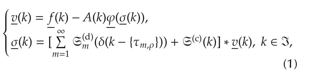
where I={0,1,2,...}the set of nonnegative integers,the vectors of reference inputerrornonlinear gainand outputhave each dimension r;and “∗”denotes convolution.Withdenoting vector/matrix transpose,the determinant of a square matrix,and I,a unit matrix(of dimension evident from the context of its usage),the other functions in(1)are defined as follows.The time-varying matrix A(k)of dimension r×ris,in general,not symmetric,and belongs to one of the following classes:i)Cp,periodic with a common fundamental period P for all the elements of A(k),i.e.,A(k−mP)=A(k)for m=...,−2,−1,0,1,2,...and for all k ∈ I;and ii)Ca,aperiodic.For simplicity and convenience in the proof of the results,we assume that the elements amn(k)of A(k)assume values such that A(k)is positive definite(we write A(k)≻0)for k∈I.Note that such an assumption is a generalization of the assumption typically made in the stability analysis of SISO time-varying feedback systems with G(z)as the Z-transform of the forward block and for which the scalar feedback timevarying gain a(k)is assumed to take values in[0,∞).When,however,there is a need to consider,in the case of linear SISO systems,the gain a(k)∈ [−a,∞),for constantthe SISO system can be transformed to an equivalent SISO system with the modified transfer functionof the forward block,and with the modified time-varying gainThe same transformation holds for the nonlinear SISO system also.See below for an analogous transformation for the MIMO system under consideration when A(k)is not positive definite.

The impulse response of the linear forward block contains two components:1)the discrete-time r×r real matrix function S(c)(k)for k∈I;and 2)the discrete-time r×r real sequence of matrix functions,one typical matrix of the sequence beingwhere the argument(δ(k−{τm,η}))indicates that a matrix of the sequence has elements which are functions of delta functions,indices m and η referring,respectively,to the matrix sequence number and sub-sequence number of the delta function in the element of the matrix itself.More specifically,the(ι,ς)th element ofis given bywhere sm,(ι,ς),ηis the coefficient of delta functions,and ρ(ι,ς)is the number of delta functions in the(ι,ς)th element.The convolution operation involving the discrete-time matrix sequence in(1),i.e.,which can be used to account for initial conditions,gives as the ℓ th element,

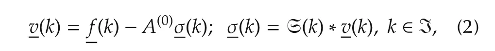
where A(0)is the matrix A(k)with its elements replaced by constant gains with values in[0,∞).Further,as a step towards analyzing the stability of(1),we also analyze the stability of the linear periodic matrix-gain MIMO system:

The proposed framework for the latter stability problem is the same as for the former.The system described by(1)is said to be ℓ2-stable ifforand an inequality of the typeholds where C is a constant.This definition is valid for(2)and(3),as also for their gain-transformed conterparts(Appendices 0.a and 0.b).

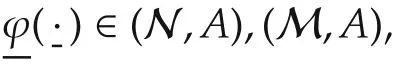
Main assumptions[A1]:The solutions to(2)are inwhich implies that the zeros of|I+A(0)Γ(z)|lie strictly inside the unit circle(i.e.,|z|＜1)of the complex plane.[A2]:A(k)≻0,k∈I;[A3]:The class(M,A)⊂(N,A)of monotone nonlinearites is defined by

We first make the following observation:the transition from either of nonlinearity classes(N,A)and(M,A)in system(1)to linearity in system(3)is abrupt.As a consequence,if we try to specialize or reduce the stability theorems meant for(1),with the above classes of nonlinearities,so as to be applicable to(3),then we find that the stability conditions so obtained for the latter system are more conservative than can be obtained by directly considering the latter system.A similar observation holds(with minor changes)to the reduction of the stability results meant for the system(1)with the nonlinearity class(N,A)to those applicable to the same system,but with the nonlinearity class(M,A).

Overview of resultsWe establish frequency-domain stability conditions for systems(1)and(3)by employing a combination of the extended discrete Parseval theorem(in Z-transform theory)and certain(matrix-)algebraic inequalities.The common strand of motivation for the theorems is the frequency-domain interpretation of the Nyquist criterion for linear time-invariant C-SISO feedback systems,in terms of the real part(designated,in what follows,by ℜ)of the product of a multiplier function and the forward block’s transfer function(see[52,53]).Theorem 1 is further motivated by the counter-intuitive properties of matrices:i)the product of two positive definite matrices need not necessarily be positive definite;and ii)the product of a positive definite matrix and an indefinite matrix can be positive definite.For instance,the product of the positive definite matricesandis sign indefinite,but the product of the positive definite matrixand the sign indefinite matrixis positive definite.

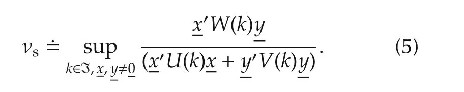
The first new inequality involves the ratios of(standard and)bi-quadratic forms:in terms of which the bi-quadratic formsatisfies the inequalitywhere the(constant)characteristic parameter(CP)νs＞ 0 is defined by

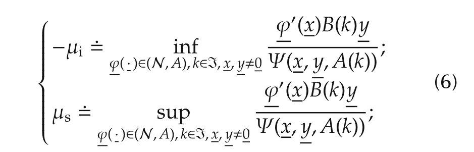
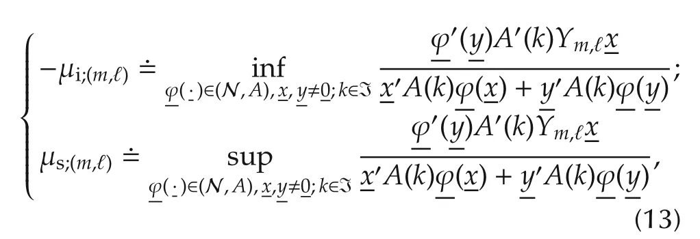
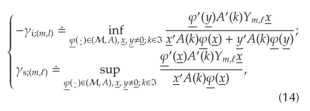
The second set of new inequalities concerns the ratios of pseudo bi-quadratic forms with vector nonlinearities and is defined as follows:i)where the CPs μi＞ 0 and μs＞ 0 are defined by

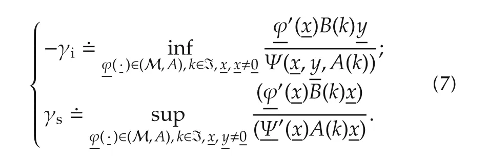
Note that the CPs νs,γi,μi,μs,γiand γsare obtained as solutions to an optimization problem(with(N,A)or(M,A)as specified),as made explicit in(5)and(7),in terms of generalized eigenvalues.

The stability conditions in Theorems 1–7 are expressed in terms of the following:i)the positive definiteness of ℜ(Y(jω))Γ(jω),where Y(jω)is the multiplier matrix frequency function,see(8)and(9)below,while noting that,in Theorem 1,Y(jω)is a constant matrix,denoted by Q∗,and ii)certain constraints onto be specified later.For simplicity in the proof of stability theorems,we assume that the generalized feedback gain is allowed to assume values in[0,∞).The stability conditions which are derived in terms of Γ(z)andcan then be specialized to“finite-gain”systems by the following algebraic operations(Appendices0.aand0.b):Replaceboth the transfer function of the forward block and the feedback by their corresponding gain-transformed versions.See Table 1 for a summary view of the new results and their domains of applicability.For stability conditions applicable to other classes of nonlinearities,see Appendix 8.

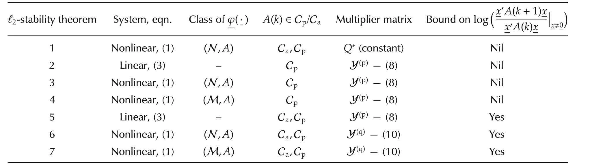
Table 1 Summary of some of the basic properties of the theorems.

3 Mathematical preliminaries

For any real-valued vector functionon I and any T∈I,the truncated functionis defined as follows:for k∈I;andfor k∉I or for I ∍ k ＞ T.Further,let ℓ2ebe the space of those real-valued functionson I whose truncationsbelong to ℓ2[0,∞)for all T ∈ I.When we first assume an infinite escape time for the solution to the system with,we imply that the solution belongs to ℓ2e.Then,it is shown that,under certain conditions on A(k)and on Γ(z),the solution actually belongs to ℓ2[0,∞).

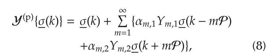
The matrix operator Y,needed to establish stability conditions for(1)and for the special cases of(2)and(3),has a(matrix)pulse response representation with elements inFor both systems(3)and(1)with A(·)∈ Cp,a typical multiplier operator Y(p)has a specific form:

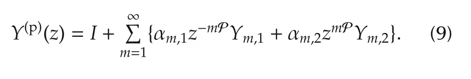
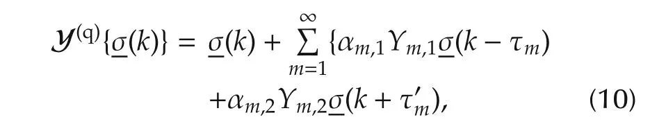
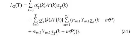
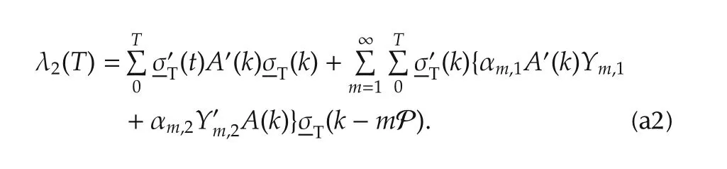
On the other hand,for(3)and(1)with A(·)∈ Ca,a typical multiplier operator Y(q)has the following form:where{αm,1,αm,2,...},{Ym,1},{Ym,2},m=1,2,...,are the same as for the multiplier operator Y(p)in(8),and sequences{τm}andare in[0,∞).Its Z transform is given byNote that Y(p)(z)and Y(q)(z)are non-positive real matrix functions.

In the proof of the stability theorems,the CPs defined above will assume different subscripts and superscripts,depending on the matrices that replace U(k),V(k),W(k)in(5);and A(k),B(k)in(6)and(7).With respect to(3),letandwhereandare vectors(of compatible dimension with A(k)).The CP of A(k)is defined by

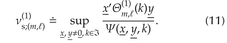
When the multiplier(8)is chosen withandwhich is skew-symmetric,the CPis re-labelled for clarity as

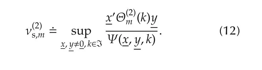
where μi;(m,ℓ)＞ 0 and γi;(m,ℓ)＞ 0,ℓ=1,2.

Remark 1The above CPs are needed in Theorems 2–7 as follows:in Theorems 2 and 5;andin Theorems 3 and 6;in Theorems 4 and 7.In general,andFurther,note the difference between the numerator ofin(13)and ofin(14):in the former,the argument ofis y,and in the latter,the argument of the same function is x.An application of the theorems to a specific problem requires computation of the CPs,which can be achieved only from a knowledge of A(k)and Ym,ℓ.

4 Main results-1:A(k)∈Caand Cp

Recall the assumptions that A(k)≻0 and A(k)is not(necessarily)symmetric for k∈I.In what follows,we employ square-bracketed numbers with prefix “H-”for the conditions(or hypotheses)in the theorems.The proofs of Theorems 1–4 depend on the correspondingly numbered lemmas(which are proved in the appendices).

Theorem 1(New circle criterion)System(1)with A(k)∈Caor Cpandis ℓ2-stable,if[H-1]:there exists a constant matrix Q∗such thatforand[H-2]:ℜQ∗Γ(z)||z|=1≻ 0.

Corollary T2-2If,in Theorem 2,andis identically a zero matrix for k∈ I,i.e.,0,k∈I,then condition[H-1]is trivially satisfied.

Theorem 3System(1)with A(k)∈ Cpand(N,A)isℓ2-stable,if[H-1]:there exists a multiplier operator Y(p)defined by(8),such that,withanddenoting,respectively,the positive and negative coefficients from the setand[H-2]:and

Theorem 4System(1)withand A(k) ∈ Cpis ℓ2-stable,if[H-1]:there exist a multiplier matrix-operator Y(p)defined by(8)and having αm,1＜0 andαm,2＜0form=1,2,...,suchthatand[H-2]:and

4.1 Proofs of stability theorems

The proofs of the above stability theorems depend on i)an application of an extended Parseval theorem(for vector functions),and ii)establishing positivity conditions for two blocks in cascade:i)for system(3),the first block is linear having Y(jω)as its transfer function,and the secondis A(k);and for system(1),the first block is the same,but the second is

Lemma 1With A(k)∈ Caor Cp,and Q∗a constant matrix,the following inequality holds:

Lemma 2With the operator Y(p)defined by(8),A(k)∈Cp,the following inequality holds:

Corollary L-1With i)the operator Y(p)defined by(8);and ii)withYm,m=1,2,...,inequality(16)of Lemma 1 is satisfied under the condition of Corollary T1-1 that replaces condition[H-1]of Theorem 1.

Lemma 3With the operator Y(p)defined by(8),A(k)∈ Cpandthe following inequality holds:

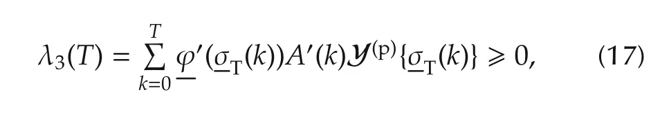
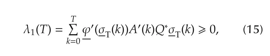
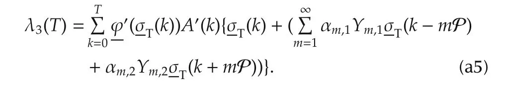
Lemma 4With the operator Y(p)defined by(8),A(k)∈Cp,and λ3(T)defined by(17),the inequality λ3(T) ≥ 0 holds for allin the domain of Y(p)and for all T∈I,if condition[H-1]of Theorem4 is satisfied.

Below we outline only the proofs of Theorems 1–3 which are based on Lemmas1–3,respectively.The proof of Theorem 4 can be obtained by a slight modification of the proof of Theorem 3.For the proofs of Lemmas 1–4,see Appendices 1–4.Let G denote the matrix operator of the forward linear block,i.e.,

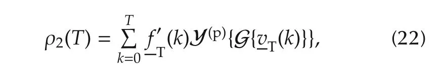
Proof of Theorem 1Consider,for a constant matrix Q∗and any T∈I,the summation

which,on invoking(1),becomes

The first summation on the right hand side of(19)can be shown,by condition[H-2]of Theorem 1 in association with the extended Parseval theorem,to satisfy the inequality

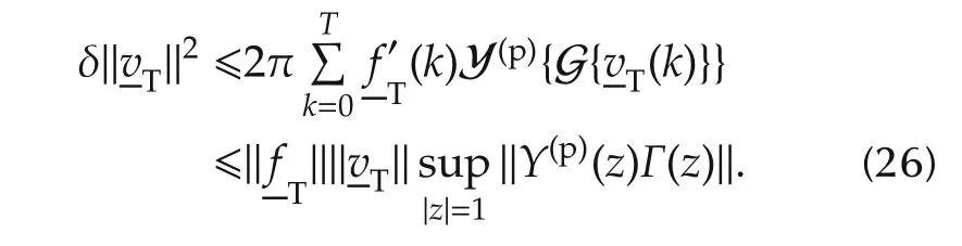
for some δ＞0.The second summation on the right hand side of(19)is non-negative by invoking Lemma 1(which is based on condition[H-1]of the theorem).Therefore,we get

The theorem is proved.

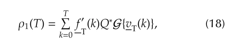
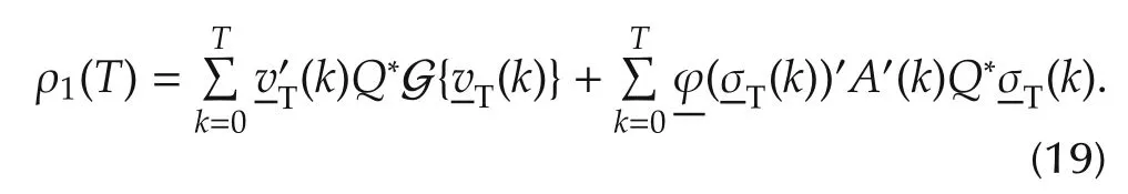
Proof of Theorem 2With the operator Y(p)defined by(8),consider,for any T∈I,the summation

on invoking(3),becomes

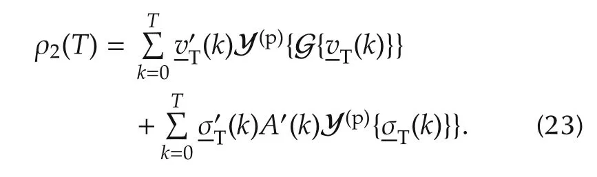
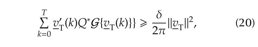
The first summation on the right hand side of(23)can be shown,by condition[H-2]of Theorem 1 in association with the extended Parseval theorem,to satisfy the inequality

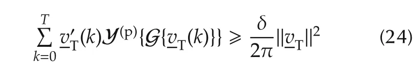
for some δ＞0.The second summation on the right hand side of(23)can,by virtue of(8),be rewritten as

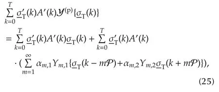
which can be shown,by invoking Lemma 1,to be nonnegative if condition[H-1]of Theorem 1 is satisfied.Finally,by applying the extended Parseval theorem to(22),and combining the result with(24),we get

Proof of Theorem 3With the operator Y(p)defined by(8),consider,for any T∈I,the summation(22)which,on invoking(1),becomes

As in the proofs of Theorems 1 and 2,the first summation on the right hand side of(27)can be shown,by condition[H-2]of the theorem,to satisfy the inequality

for some δ＞0.After replacing Y(p)in the second summation of the right hand side of(27)by the right hand side of(8),we proceed along the lines of the proof of Theorem 1 above.Finally,we invoke Lemma 2 along with conditions[H-1]and[H-2]of the theorem to complete the proof.

Remark 3In system(1),we have assumed,for clarity,transparency and simplicity in the derivations,a separable structure for the time-varying nonlinearity,viz.,For nonseparable nonlinearities(written typically asTheorems 1,3 and 4 need to be recast after suitable changes in the definitions of classes(N,A)and(M,A)in the statement of lemmas(related to Theorems 1,3 and 4)and in the proofs of those lemmas.

Remark 4In Theorems 1,3 and 4,the stability conditions for system(1)withneither entail any restriction on the rate of variation of A(k),nor assume path-independence line integrals(i.e.,PILI property)ofFurther,if the coefficientsare not all negative,then Theorem 3 holds only for the class(Mo,A)⊂(M,A)of odd-monotone nonlinearities.

Remark 5General multivariable nonlinearities of the type considered here are too general to be amenable for computation of their CP’s in the illustration of theorems in Section 4 below.Alternatively,we interpret the time-domain constraints(of the theorems)on the multiplier matrix in terms of bounds on the CPs themselves,μi;(m,ℓ)and μs;(m,ℓ)defined by(13),and γi;(m,ℓ)and γs;(m,ℓ)by(14),once the frequency-domain(i.e.,real-part)conditions involving the Z transform of the multiplier and the system function Γ(z)for|z|=1 are satisfied.

5 Main results-2:A(k)∈Ca

When A(k)∈ Ca,Theorems 2–4 are inapplicable.Further,if Theorem 1,meant for both A(k)∈Caand Cp,is inapplicable,i.e.,we cannot find a constant matrix Q∗to satisfy the conditions of Theorem 1,our goal is to establish the constraints,if any,on the local/global rate of variation ofA(k)for the stability of systems(1)and(3).To this end,we define the class B of scalar functions ω(·)such that ω(k)for k ∈ I,withand generalize Lemma 5 of[16,Pages 633,638–640]so as to be applicable to(time-varying)matrix gains.

With ω(·)∈ B,by the statement that e−ξkω(k)A(k)is non-increasing some non-negative ξ,we mean that,for k∈I,

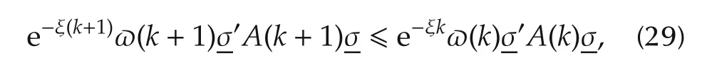
which can be reduced to the following inequality:

Along similar lines,by the statement that ω(k)eζkA(k)is non-decreasing for some non-negative ζ,we mean that

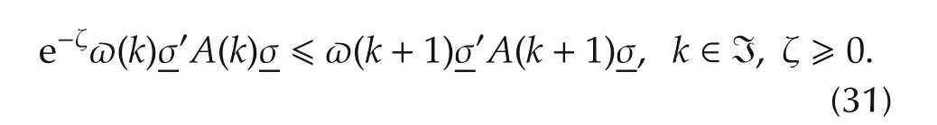
Recalling that A(k)≻0 for k∈I,it can be shown that(30)and(31)together reduce to the following inequality:

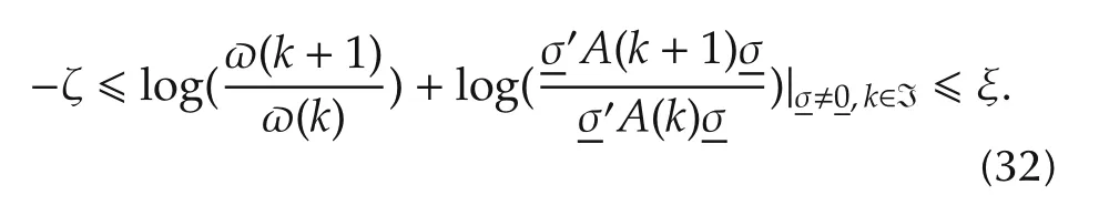
In order to arrive at explicit conditions on A(k)to satisfy(32),we need to find functions ϑa(k)andϑb(k),k∈I as solutions to the following generalized eigenvalue problem(which is of independent interest by itself in function-optimization):

In effect,we are looking for a solution to the following problem at each “frozen”instant,k′∈ I:

We now state Theorems 5–7 and the lemmas needed to prove them.Theorem 5 concerns system(3);and Theorems 6 and 7,system(1)with,respectively,and(M,K).For Theorem 5,the multiplier matrix is given by(8),where P is replaced by p,which is treated as an additional parameter to be chosen.On the other hand,for Theorems 6 and 7,we choose the multiplier operator Y(q)defined by(10).As in Section 4(for Theorems 2–4),the CPs of A(k)andthat appear in Theorems 5–7 below areanddefined above,respectively,by(11),(13)and(14).We note the following:if A(k)∈Cpand P=p,then Theorem 2 comes into play,which implies that there is no restriction on the rate of variation of A(k)and no need for Theorem 5.

Theorem 5System(3)with A(k) ∈ Cais ℓ2-stable if there exist a multiplier matrix-operatordefined by(8)with P replaced by parameter p;function ω(·)∈ B as defined above;and nonnegative constants,ξ,ζ,such that[H-1]: ω(k)e−ξkA(k)is non-increasing and ω(k)eζkA(k)is non-decreasing for k ∈ I;[H-2]:and,for some ε＞0,[H-3]:∞;and

The proof of Theorem 5,which depends on the following lemma,is omitted due to both lack of space and its similarity to the proof of Theorem 2 above,in partial combination with the proof of Theorem 1 in[16,pages 630–631,640–642].

Lemma5With the operator Y(p)defined by(8)with P replaced by parameter p;ω(·)∈ B,and nonnegative constants ξ,ζ,the summation

Condition[H-1]of Theorem 5 is equivalent to appropriate bounds on the generalized eigenvalues of{A(k+1),A(k)},as made explicit by the following lemma.

Corollary L5If ω(k)e−ξkA(k)is non-increasing and ω(k)eζkA(k)is non-decreasing for all k∈ I and for some ξ ≥ 0,ζ ≥ 0,then with ϑa(k)and ϑb(k)defined in(33),i)(logϑb(k))+denoting the positive excursions of logϑb(k);ii)(logϑa(k))−denoting the negative excursions of logϑa(k)for k∈ I,then,for some positive constants N1and N2,for all finite T＞0 and k∈I,

and in addition,for ξ ≠ ζ,

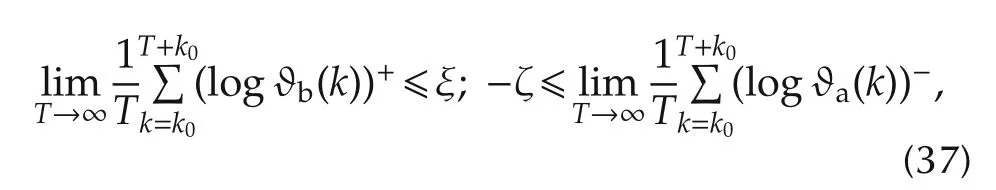
but for ξ = ζ,logϑa(k)and logϑb(k)are unrestricted.

The proof of Corollary L5 is similar to that of Lemma 1 of[16,Pages 638–640],and is hence omitted.When A(k)∈Cpwith period P≠p,then(36)and(37)reduce respectively to

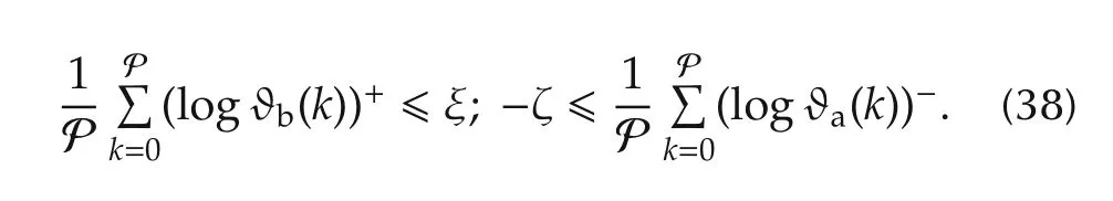
The above conditions are also equivalent to condition[H-1]of Theorems 6 and 7 below.

Theorem 6System(1)with A(k)∈ Caand(N,A)is ℓ2-stable,if[H-1]:for some non-negative ξ and ζ,and for ω(·) ∈ B, ω(t)e−ξkA(k)is nonincreasing and ω(t)eζkA(k)is non-decreasing,[H-2]:there exists a multiplier operator Y(q)defined by(10),such that,withanddenoting,respectively,the positive and negative coefficients from the setand,for someand ℜY(q)·(e−εz)Γ(e−εz)||z|=1≻ 0.

Lemma 6With the operator Y(q)defined by(10),A(k)∈ Ca,and ω(·) ∈ B,the following inequality holds:

Due to lack of space,the proof of Theorem 6 is not given here(It is similar to the proof of Theorem 1(for SISO systems)in[16]after invoking the above Lemma 6 which is proved in Appendix 6).

Theorem 7System(1)with A(k)∈ Caand(M,A)is ℓ2-stable,if[H-1]:for some non-negative ξ and ζ,and ω(·)∈ B,ω(k)e−ξkA(k)is non-increasing and ω(k)eζkA(k)is non-decreasing;[H-2]:there exist a multiplier matrix-operator Y(q)definedby(10)withαm,1＜ 0 and αm,2＜ 0,such thatand for someand

The proof of Theorem 7 requires the following lemma(proved in Appendix 7).

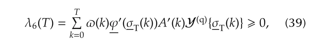
Lemma 7With i)the operator Y(q)defined by(10)with αm,1＜ 0 and αm,2＜ 0,ii)and(iii)ω(·)∈ B,inequality(39)holds for allin the domain of(10)and for all T ∈ I,if conditions[H-1]–[H-3]of Theorem 7 are satisfied.

Remark 6Theorems 5–7(and their lemmas)are applicable to the case of A(k)∈Cpby substituting mP for both τmandIn this case,the stability constraints(36)and(37)on the generalized eigenvalues of{A(k+1),A(k)}can be converted to equivalent constraints over an interval P,as explicitly set forth in Corollary L5 above for system(3)with A(k)∈Cp.Note that no reference is made to dwell-time aspects of A(k).A-part from the above,ifis odd-monotone,then the constraint of negativity on αm,1,αm.2for m=1,2,...,in Theorems 4 and 7 can be removed.

Remark 7In continuation of Remark 4 earlier(concerning Theorems 1,3 and 4),Theorems 6 and 7 for system(1)can be generalized to hold for nonlinearities with i)a slope restriction or/and ii)the PILI property ofTo this end,in the definitions of thewhere ℓ=1,2,and ofthe desired constraint on the slope matrixof the nonlinearities can be included as constraints,without leading to any extra terms in the frequency domain inequality condition[H-3]in those theorems.Note that such extra terms are typical of the literature on C-SISO systems(with a constraint on the derivative of the nonlinearity),see[15,54].A similar comment is applicable to the inclusion of the PILI property in the definition of the CPs.

6 Comparison with Literature

2)Except for[27],which contains an extension of the Popov-related criterion of[26],the latter using the the multivariable form of the Lur’e-Postnikov Lyapunov function for time-invariant,monotone non-decreasing nonlinearites to time-invariant diagonal MIMO nonlinearities,to slowly time-varying,rate-and sectorrestricted,diagonal MIMO nonlinearities,there seem to be no results in the literature coresponding to Theorems 3,4,6 and 7 of the present paper,as applied to nonlinear and time-varying D-MIMO systems.Note that in Theorem 6(meant forof the present paper,no restrictions are imposed on the derivative of the nonlinearity.Even when Theorem 6 is specialized to D-SISO systems,it significantly improves the circle criterion or Popov-type results of[26,31]and others,while acting as a complement to the D-SISO results of[16]which deals with time-varying monotone and odd-monotone nonlinearities.The continuous-time counterpart of Theorem 6,generalizing the celebrated Popov criterion[11]for timeinvariant C-SISO systems and applicable to time-varying systems also,is expected to appear elsewhere.

3)Theorems 3,4,6 and 7 are not mere discretizations of the theorems of[22]for C-MIMO systems,but,on the contrary,are significantly different from them on the following counts:i)forno PILI property is assumed here,and the multiplier function Y(z)contains terms involving powers of z and z−1and hence is more general than the multiplier function of Theorem 4B for C-MIMO systems in[22]which contains only one term with(the complex variable)s;ii)forthe bound on the norm of Y(z)as proposed in Theorem 4A of[22],is replaced by a bound on the CPs of the nonlinearity itself;and iii)the latter improvement can be translated to C-MIMO systems within[22],but the former improvement,i.e.,item i),cannot,without the assumption of PILI property for the nonlinearity.

4)In Theorem 3,there are no constraints either on the slope of the nonlinearity or on its monotonicity.Therefore,it is a significant generalization of the results of the literature on the stabiliy of nonlinear,time-invariant DMIMO systems.We can,of course,insert any required constraint on the slope of the nonlinearity(in the class(N,A))in the optimization process,made explicit in(13),to extract the CP of the actual nonlinearity under consideration.The consequence is that the magnitude of μs;(m,ℓ),ℓ=1,2 becomes smaller than the one without a slope constraint on the nonlinearity.A further distinctive property of the theorem is that such an inclusion of the constraint on the slope of the nonlinearity does not lead to the addition,in the multiplier function,of a term involving a quadratic function of Γ(jω)(Note that a magnitude square of the transfer function of the forward block appears in the multiplier functions of the literature for nonlinear,time-invariant D-SISO systems).It is instructive and interesting to compare Theorems 3 and 4.Note that γs;(m,ℓ)＜ μs;(m,ℓ),ℓ=1,2.Also,if the characteristic propertes of a single-variable monotonic nonlinearity are any guide,the γi;(m,ℓ)is conjectured to be small(in contrast with μi;(m,ℓ),ℓ=1,2,defined by(13)forwhich could be quite large).

5)In an application of the theorems,the elements of the matrices and their coefficients are to be so chosen as to minimize the CPs,while simultaneously satisfying the real part condition of the corresponding theorems.

7 Illustration of Theorems 1–7

A note of caution is in order here.For crossverification and for pedagogical reasons,it is advisable to check the numerical results and the inferences that follow from them.

Application of Theorem 1With Q∗=[(0.5,−0.6);(−0.3,0.8)],it can be verified that condition[H-2]is satisfied,but not[H-1]for the above A(k).In fact,Note that,in the present case,bothand Q∗are both positive definite,but their product is not(This is one of the reasons for the C-MIMO and D-MIMO stability criteria to be not just matrix extensions of C-SISO and D-SISO stability criteria,respectively).Therefore,Theorem 1 cannot be applied to this case.However,with Q∗=[(0.617,−0.5);(0.0,0.473)],it can be verified that not only condition[H-2]is satisfied,butandTherefore,for the special case ofi.e.,for system(3),we can apply Theorem 1 to conclude that the system is stable for any type of switching between A1and A2.No such inference(from Theorem 1)can be drawn for system(1),unlesssatisfies the condition[H-1]of the theorem for the prescribed A1and A2,i.e.,

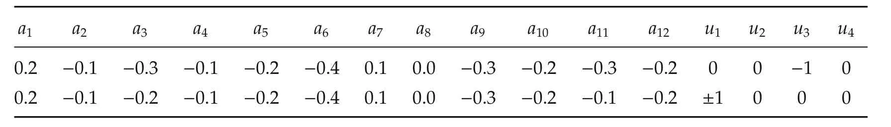
Table 2 Values of coefficients(am,m=1,2,...,12)and(u1,u2,u3,u4)of Ye(z)to satisfy the real-part condition of the theorems.

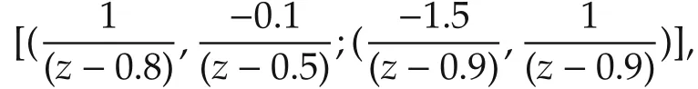
The two multiplier functions reduce respectively to the following:i)Multiplier Functionwhere Q0=[(1.0,−0.4);(0.1,0.5)]and Q1=[(0.2,0.2);(0,0.3)](Weidentifythecoefficient(−1)ofQ1with αm,1in Theorems 3 and 6).ii)Multiplier Functionwhere Q0=[(0.6,−0.6);(0.0,0.5)]and Q1=[(0.2,0.0);(0.1,−0.3)](Here,we identify the coefficient(+1)of Q1with αm,2in Theorems 3 and 6).

Application of Theorems 2–7This involves the computation of the CPs of A(k)andFor the former,is defined by(11);and for the latter,whendefined by(13);and when ϕ(·)∈(M,A),(Mo,A),the pair(γs;(m,ℓ),γi;(m,ℓ))(ℓ=1,2)is defined by(14).It is to be noted that,in the computation of the CPs,A′(k)is to be replaced by A′(k)Q0and A′(k)Ym,1by A′(k)Q1.Note that i)and,see Remark 2 in Section 3,and ii)the conditions[H-2]of Theorems 2–4 and conditions[H-3]of Theorems 5–7 are satisfied for both the multiplier functions.What remains is the verification of the other conditions of the theorems.

1)Multiplier function F1(z):Note that α1,1= −1 as the coefficient of Q1z−1.Since the multiplier function contains only the z−1term,for A(k)∈ Cp,P=1,which means that A(k)must be a constant matrix.Therefore,an application of Theorem 2 to the linear system with A(k)∈Cpis not interesting.However,for the same constant A(k),we can invoke Theorem 3 forand Theorem 4 forOn the other hand,we can apply Theorem 5 for A(k)∈Ca,and Theorems 6 and 7 forand(M,A),respectively.The results are presented below.

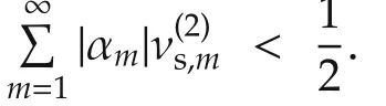
[Theorem 3]:The nonlinear system with a constant matrix gain andis stable,if μs;(1,1)＜ 0.5.

[Theorem 4]:The nonlinear system with a constant matrix gain andis stable,if(γs;(1,1)+γi;(1,1))＜ 0.5.

[Theorem 5]:Note that p=1.Condition[H-2]of the theorem implies that the linear system(3)is stable,if there exists a constant ξ ＞ 0 such that(The last inequality is invalid,if.And this fact is a guiding factor in the choice of the multiplier matrix).We can effect a trade-off between ξ andwhile guaranteeing the stability of the linear system.Further,with the chosen value of ξ,condition[H-1]of Theorem 4 can be written explicitly in terms of the rate of variation of A(k)by invoking Corollary L5 of Theorem 5.We compute the CP of A(k)from(11),with,as indicated above,A′(k)replaced by A′(k)Q0and A′(k)Ym,1by A′(k)Q1,to getwhere the first argument in max corresponds to A1and the second,to A2.From condition[H-2]of Theorem 5,the linear system is stable if we set,for instance,ξ=0.5893,and invoke Corollary L5 to make explicit the constraints on switching.To this end,let ϑb(k′)of(34)correspond to the transition from A1to A2at instant,say,k′;and ϑb(k′′)of(34)to the transition from A2to A1at instant,say,k′′.It is found that ϑb(k′)=5.9666,and ϑb(k′′)=3.4083.Since the multiplier does not contain z and/or higher powers of z,the exponent ζ that appears in condition[H-1]of Theorem 5(as also of Theorems 6 and 7)does not exist,and can be set to an arbitrarily large number.Further,in any finite interval of time accommodating an integral number of switchings,the difference between the numbers of transitions from A1to A2and vice versa is at most 1.If the average number of transitions in a unit interval from A1to A2or vice versa is denoted by n,we conclude,by invoking Corollary L5,that the system is stable,if the first inequality of each of(36)and(37)is satisfied.This procedure leads to the deciding inequality,(log5.9666+log3.4083)n≤ξ=0.5893,from which we get n＜0.1956.If it is the case that A(k)is,in fact,periodic with period P,i.e.,A(k)∈Cp,then in an interval of P,the number of transitions from A1to A2or from A2to A1is less than 0.1956P for system stability.An interesting byproduct is that Theorem 5 guarantees,in a non-trivial sense,stability of the linear system for switchings between A1and A2,if P＞5 units.However,in situations,where P＜5,i.e.,at least one switching cannot take place in an interval of P,then Theorem 5 is not relevant for A(k)∈Cp,unless the switching matrices A1and A2are such thatand the maximum of the generalized eigenvalues of the matrix pairs(A1,A2)and(A2,A1)are reduced.In other words,there is a minimum period of A(k)∈Cpfor which Theorem 5 gives non-trivial results for stability.

[Theorems 6 and 7]:Assume that we have chosen ξ=0.5893,as obtained above from an application of Theorem 5.The nonlinear system(1)with A(k)∈Cais stable for i)having its CP μs;(1,1)＜ 0.3568;andii)having its CP sobeying the inequality(γs;(1,1)+γi;(1,1))＜ 0.3568(In both the cases,we need the explicit forms ofto compute their CPs).

While the constraints on the rate of variation of A(k)are the same as the ones obtained from an application of Theorem 5 to the example,those on the nonlinearity(in Theorems 6 and 7)are more severe than the ones presented above as application of Theorems 3 and 4 to the case of A(k)being a constant matrix.Continuing with the comments made above on optimizing the multiplier for application of Theorem 3 to the system under consideration,if μs;(1,1)is made as small as possible in both the cases offor Theorem 6,and offor Theorem 7,then a larger ξ,which refers to the rate of variation of A(k),can be traded for the smaller μs;(1,1)in Theorem 6,and for the smaller γs;(1,1)and γi;(1,1)in Theorem 7.

2)Multiplier function F2(z):Note that α1,2=+1 as the coefficient of Q1z.With A(k)∈Caand A1,A2and the scheme of switching between them as assumed above,we note thatandin this case,too.Since the multiplier function contains only the z term,for A(k)∈Cp,P=1,which means that A(k)is a constant matrix.As with the multiplier function F1(z),an application of Theorem 2 to the linear system with A(k)∈Cpis not interesting.However,we can employ Theorems 3 and 6 forand Theorem 5 for A(k)∈Ca.We can apply Theorems 6 and 7 only for the case ofthe odd-monotone class of nonlinearities.Note also that,while applying Theorems 3 and 6 forthe CP μi;(1,2),defined by(13)forcomes into play.

[Theorem 3]:The nonlinear system with a constant matrix gain andis stable if μi;(1,2)＜ 0.5.

[Theorem 4]:The nonlinear system with a constant matrix gain andis stable if(γs;(1,2)+γi;(1,2))＜ 0.5.

[Theorem 5]:Since p=1,condition[H-2]of the theorem implies that the linear system(3)is stable if there exists a constant ζ ＞ 0 such that(As with the application of F1(z)above,the last inequality is invalid,ifWe can effect a trade-off between ζ andwhile guaranteeing the stability of the linear system.Further,with the chosen value of ζ,condition[H-1]of Theorem 5 can be written explicitly in terms of the rate of variation of A(k)by invoking Corollary L5 of Theorem 5.We compute the CP of A(k)from(11),with,as indicated above,A′(k)replaced by A′(k)Q0and A′(k)Y1,2by A′(k)Q1,to getwhere the first argument in max corresponds to A1and the second,to A2.From condition[H-2]of Theorem 5,the linear system is stable if we set,for instance,ζ=0.3735,and invoke Corollary L5 to make explicit the constraints on switching.We compute,in the present case,ϑa(k′)and ϑa(k′′)as defined by(34):ϑa(k′)=0.2935,and ϑa(k′′)=0.3955.Since the multiplier does not contain z−1and/or higher powers of z−1,the exponent ξ that appears in condition[H-1]of Theorem 5(as also of Theorems 6 and 7)does not exist,and can be set to an arbitrarily large number.

If the average number of transitions in a unit interval from A1to A2or vice versa is denoted by n,we conclude,by invoking Corollary L5,that the system is stable,if now the second inequality of each of(36)and(37)is satisfied.This procedure leads to the deciding inequality,(log0.2935+log0.3955)n≥ −ζ= −0.3735,from which we get n＜0.1734.

If it is the case that A(k)is,in fact,periodic with period P,i.e.,A(k)∈Cp,then in an interval of P,the number of transitions from A1to A2or from A2to A1is less than 0.1734P for system stability.In a non-trivial sense,the linear system is stable for switchings between A1and A2,if P＞6 units.For P＜6 units,Theorem 5 is not relevant,unless the switching matrices A1and A2are such thatand the maximum of the generalized eigenvalues of the matrix pairs(A1,A2)and(A2,A1)are reduced.

[Theorems 6 and 7]:Assume that we have chosen ζ=0.3735,as obtained above from an application of Theorem 5.The nonlinear system(1)with A(k)∈Cais stable for i)having its CPand ii)having its CPs obeying the inequalityIn both the cases,we need the explicit forms of ϕ(·)∈ (N,A),(Mo,A)for computation of their CPs.Comments made above on the use of the multiplier function F1(z)in Theorems 6 and 7 hold here,too,with appropriate changes,wherever required.

7.1 D-SISO system stability as a special case

In order to exhibit the novelty of the stability theorems of the present paper,as specialized to D-SISO systems,and for the sake of completeness,we consider Example 1 of[14],dealing with the asymptotic stability of a time-invariant nonlinear D-SISO system.

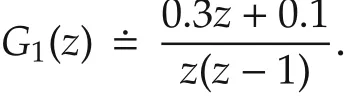
The multiplier(1+ α1z−1+ α2z),where α1and α2are constants to be chosen,needs to first satisfy the real part conditions of the theorems.We then invoke the remaining conditions of the theorems to determine the constraints,if any,ona(k)and ϕ(·)for the stability of the system under consideration.1)α1=−0.5;α2=0.0;¯a=6.603.Theorem 2 is inapplicable,because the multiplier contains only z−1,and P=1(as in the case of Example 1 considered above,using the multiplier function F1(z)).

In contrast,Theorem 5 is applicable,as are Theorems 3,4,6 and 7,along lines similar to those of Example 1 above for the multiplier F1(z).To give one interesting result,we conclude,from an application of Theorem 6,that the time-varying nonlinear D-SISO system withis stable for values of ξ and μs;(1,1)satisfying the inequality,(1+eξ)μs;(1,1)＜ 2.As explained in Example 1 above,we can strike a trade-off between ξ and μs;(1,1),and impose,on the logarithmic rate of variation of a(k),a global upper bound,if a(k)∈Ca,or an average(over a period)bound,if a(k)∈Cp.No such results are available in the literature even for D-SISO systems.2)α1=−0.99;α2=0.0;¯a=7.4.Further analysis is similar to that with the first multiplier,except that the constraints on ξ,CPs and the corresponding trade-offs are much narrower.This is because|α1|≈ 1.Similar comments(with changes,mutatis mutandis)apply to multipliers with the parameters,(α1=0.0,α2=0.893,¯a=9);and(α1=0.0,α2=0.9895,¯a=9.9),for both of which the analysis follows that of the D-MIMO example above in the case of the multiplier F2(z).

8 Conclusions

We have derived new frequency-domain conditions for the ℓ2-stability of D-MIMO systems,consisting of a linear time-invariant block in the forward path and a time-varying periodic/aperiodic matrix gain with a vector nonlinearity in the feedback path.The classes of nonlinearity considered are non-monotone and monotone,but with no assumption of path-independence of their line integrals and with no slope restrictions.The stability conditions are expressed in terms of the positive definiteness of the real part of the matrix product of the transfer function of the linear forward block and a matrix multiplier function.For periodic A(k),the choice of one class of multiplier functions(to satisfy the real part condition of the theorems)imposes no constraints on the rate of variation of A(k).However,for aperiodic A(k),a more general multiplier function leads to constraints on certain global averages of the generalized eigenvalues of(A(k+1),A(k)),k=1,2,....Significantly,no reference is made to dwell time(average or otherwise)structure of the matrix gains.A comparison with the results of the literature on D-MIMO systems shows the novelty and superiority of the stability conditions of the new theorems.Two illustrative examples,one each for D-MIMO and D-SISO systems,complete the paper.An open problem is to find suitable Lyapunov-function candidates for establishing(and possibly refining/generalizing)Theorems 2–7.

[1] A.I.Lur’e,V.N.Postnikov.On the theory of stability of control systems.Prikladnaya Mathematika i Mekhanika,1944,8(3):246–248.

[2]R.Shorten,F.Wirth,O.Mason,et al.Stability criteria for switched and hybrid systems.SIAM Review,2007,49(4):545–592.

[3] H.Lin,P.J.Antsaklis.Stability and stabilizability of switched linear systems:a survey of recent results.IEEE Transactions on Automatic Control,2009,54(2):308–322.

[4]D.Liberzon.Switchingin Systemsand Control.Boston:Birkhauser,2003.

[5]S.Sun,S.S.Ge.Switched Linear Systems:Control and Design.Berlin:Springer-Verlag,2005.

[6] G.Szego.On the absolute stability of sampled-data control systems.Proceedings of the National Academy of Sciences of the United States of America.1963,50(3):558–560.

[7]K.Premaratne,E.I.Jury.Discrete-time positive-real lemma revisited: the discrete-time counterpart of the Kalman-Yakubovitch lemma.IEEE Transactions on Circuits and Systems–I:Fundamental Theory and Applcations,1994,41(11):747–750.

[8]Y.Yamamoto.A function space approach to sampled-data control systems and tracking problems.IEEE Transactions on Automatic Control,1994,39(4):703–712.

[9] Y.Z.Tsypkin.On the stability in the large of nonlinear sampleddata systems.Doklady Akademii Nauk SSSR(USSR),1962,145:52–55.

[10]G.Zames.On the input-output stability of time-varying nonlinear feedback systems–Parts 1 and 2.IEEE Transactions on Automatic Control,1966,11(2):228–238,465–476.

[11]V.M.Popov.Absolute stability of nonlinear systems of automatic control.Automation and Remote Control,1962,22(8):857–875.[12]Y.Z.Tsypkin.A criterion for absolute stability of automatic pulse systems with monotonic characteristics of the nonlinear element.Doklady Akademii Nauk SSSR(USSR),1964,155:1029–1032.

[13]E.I.Jury,B.W.Lee.On the stability of a certain class of nonlinear sampled-data systems.IEEE Transactions on Automatic Control,1964,9(1):51–61.

[14]R.P.O’Shea,M.I.Younis.A frequency-time domain stability criterion for sampled data systems.IEEE Transactions on Automatic Control,1967,12(6):719–724.

[15]G.Zames,P.Falb.Stability conditions for systems with monotone and slope restricted nonlinearities.SIAM Journal on Control,1968,6(1):89–108.

[16]Y.V.Venkatesh.Riesz-Thorin theorem and ℓp-stability of nonlinear time-varying discrete systems.Journal of Mathematical Analysis and Applications,1988,135(2):627–643.

[17]M.Z.Oliveira,J.M.G.da Silva Jr.,D.Coutinho.Stability analysis for a class of nonlinear discrete-time control systems subject to disturbances and to actuator saturation.International Journal of Control,2013,86(5):869–882.

[18]P.A.Bliman,A.M.Krasnosel’skii.Popov absolute stability criterion for time-varying multivariable nonlinear systems.1999:http://citeseerx.ist.psu.edu/viewdoc/summary?doi=10.1.1.27.9354.

[19]D.A.Altshuller.Delay-integral-quadratic constraints and stability multipliers for systems with MIMO nonlinearities.IEEE Transactions on Automatic Control,2011,56(4):738–747.

[20]Z.Huang,Y.V.Venkatesh,C.Xiang.On frequency-domain L2-stability conditions for a class of switched linear and nonlinear systems–Part II:MIMO.Singapore:National University of Singapore.2011:1–30.

[21]Z.Huang.Stability Analysis of Switched Systems.Singapore:National University of Singapore,2011.

[22]Z.Huang,Y.V.Venkatesh,C.Xiang,et al.Frequency-domain L2-stability conditions for time-varying linear and nonlinear MIMO systems.Control Theory and Technology,2014,12(1):13–34.

[23]M.S.Branicky.Multiple Lyapunov functions and other analysis tools for switched and hybrid systems.IEEE Transactions on Automatic Control,1998,43(4):475–482.

[24]M.Akar,K.S.Narendra.On the existence of common quadratic Lyapunov functions for second-order linear timeinvariant discrete-time systems.International Journal of Adaptive Control and Signal Processing,2002,16(10):729–751.

[25]T.Hu,Z.Lin.Absolute stability analysis of discrete-time systems with composite quadratic Lyapunov functions.IEEE Transactions on Automatic Control,2005,50(6):781–797.

[26]V.Kapila,W.Haddad.A multivariable extension of the Tsypkin criterion using a Lyapunov-function approach.IEEE Transactions on Automatic Control,1996,41(1):149–152.

[27]W.M.Haddad,V.Kapila.Robust stabilization for discrete-time systems with slowly time-varying uncertainty.Proceedings of the 34th IEEE Conference on Decision and Control.New Orleans:IEEE,1995:202–207.

[28]M.Lazar,W.P.Maurice,M.H.Heemels,et al.Lyapunov functions,stability and input-to-state stability subtleties for discrete-time discontinuoussystems.IEEE Transactionson Automatic Control,2009,54(10):2421–2425.

[29]G.Zhai,B.Hu,K.Yasuda,et al.Stability and ℓ2-gain analysis of discrete-time switched systems.Transactions of the Institute of Systems,Control and Information Engineers,2002,15(3):117–125.

[30]G.Zhai.Stability and ℓ2-gain analysis of switched symmetric systems.Stability and Control of Dynamical Systems with Applications.D.Liu,P.J.Antsaklis,eds.Boston:Birkhauser,2003.

[31]W.M.Haddad,D.S.Bernstein.Explicit construction of quadratic Lyapunov functions for the small gain,positivity,circle,and Popov theorems and their application to robust stability–Part II:Discrete-time theory.International Journal of Robust and Nonlinear Control,1994,4(11):249–265.

[32]N.S.Ahmad,W.P.Heath,G.Li.LMI-based stability criteria for discrete-time Lur’e systems with monotonic,sector-and sloperestricted nonlinearities.IEEE Transactions on Automatic Control,2013,58(2):459–465.

[33]N.S.Ahmad,W.P.Heath,G.Li.Lyapunovfunctions for generalized discrete-time multivariable Popov criterion.Proceedings of the 18th IFAC World Congress.Milano:Elsevier Science,Ltd.,2011:3392–3397.

[34]W.P.Heath,G.Li.Lyapunov functions for the multivariable Popov criterion with indefinite multipliers.Automatica,2009,45(12):2977–2981.

[35]N.Ahmad,W.Heath,G.Li.Lyapunov functions for discretetime multivariable Popov criterion with indefinite multipliers.Proceedings of the 40th IEEE Conference on Decision and Control.Piscataway:IEEE,2010:1559–1564.

[36]L.Gurwitz.Stability of discrete linear inclusion.Linear Algebra and its Applications,1995,231(1):47–85.

[37]D.Liberzon,J.P.Hespanha,A.S.Morse.Stability of switched systems:a Lie-algebraic condition.Systems&Control Letters,1999,37(3):117–122.

[38]G.Zhai,D.Liu,J.Imae,et al.Lie algebraic stability analysis for switched systems with continuous-time and discrete-time subsystems.IEEE Transactions on Circuits and Systems–II:Analog and Digital Signal Processing,2006,53(2):152–156.

[39]T.Ooba,Y.Funahashi.On the simultaneous diagonal stability of linear discrete-time systems.Systems&Control Letters,1999,36(3):175–180.

[40]T.Monovich,M.Margaliot.Analysis of discrete-time linear switched systems:a variational approach.SIAM Journal of Control and Optimization,2011,49(2):808–829.

[41]M.Margaliot.Stability analysis of switched systems using variational principles:an introduction.Automatica,2006,42(12):2059–2077.

[42]M.Margaliot,G.Langholz.Necessary and sufficient conditions for absolute stability:the case of second-order systems.IEEE Transactions on Circuits and Systems–I:Fundamental Theory and Applications,2003,50(2):227–234.

[43]A.Molchanov,D.Liu.Robust absolute stability of time-varying nonlinear discrete-time systems.IEEE Transactions on Circuits and Systems–I:Fundamental Theory Applications,2002,49(8):1129–1137.

[44]J.H.Davis.Discrete systems with periodic feedback.SIAM Journal on Control,1972,10(1):1–13.

[45]A.S.Morse.Supervisory control of families of linear setpoint controllers–Part I:exact matching.IEEE Transactions on Automatic Control,1996,41(10):1413–1431.

[46]R.DeCarlo,M.Branicky,S.Pettersson,et al.Perspectives and results on the stability and stabilizability of hybrid systems.Proceedings of the IEEE,2000,88(7):1069–1082.

[47]J.C.Geromel,P.Colaner.H∞and dwell time specifications of continuous-time switched linear systems.IEEE Transactions on Automatic Control,2010,55(1):207–212.

[48]J.P.Hespanha.Stability of switched systems with average dwelltime.Proceedings of the 38th IEEE Conference on Decision and Control.Piscataway:IEEE.1999:2655–2660.

[49]L.Zhang,P.Shi.Stability,ℓ2-gain and asynchronous H∞control of discrete-time switched systems with average dwell time.IEEE Transactions on Automatic Control,2009,54(9):2193–2200.

[50]X.Zhao,L.Zhang,P.Shi,et al.Stability and stabilization of switched linear systems with mode-dependent average dwell time.IEEE Transactions on Automatic Control,2012,57(7):1809–1815.

[51]R.W.Brockett,J.L.Willems.Frequency-domain stability criteria–Parts 1 and 2.IEEE Transactions on Automatic Control,1965,10(7/10):255–261,407–413.

[52]M.A.L.Thathachar.Stability of systems with power-law nonlinearities.Automatica,1970,6(5):721–730.

[53]Z.Huang,Y.V.Venkatesh,C.Xiang,et al.Frequency-domainℓ2-stability conditions for switched linear and nonlinear SISO systems.International Journal of Systems Science,2014,45(3):682–703.

[54]A.G.Dewey,E.I.Jury.A stability inequality for a class of nonlinear feedback systems.IEEE Transactions on Automatic Control,1966,11(1):54–63.

[55]Y.V.Venkatesh.Global variation criteria for the L2-stability of nonlinear time varying systems.SIAM Journal on Mathematical Analysis,1978,19(3):568–581.

8 April 2014;revised 4 July 2014;accepted 4 July 2014

DOI10.1007/s11768-014-4045-7

E-mail:yv.venkatesh@gmail.com.

©2014 South China University of Technology,Academy of Mathematics and Systems Science,CAS,and Springer-Verlag Berlin Heidelberg

Appendix 0.a

When the feedback block of(1)has a finite gain,i.e.,whereis the constant upper bound matrix,the stability results remain valid under a transformation of forward and feedback blocks.For clarity,we employ subscript 1 in the(dependent)variables of the equation governing the finite gain system,but retain¯A as the upper bound matrix for the feedback block in both the linear and nonlinear cases.

Linear MIMO gain transformationLet the equations of the “finite”gain linear MIMO system with the upper bound matrixbe given byThe output of the “1infinite”gain system(3)and feedback gainas a result of which the feedback output is(which is,by a quirk in the transformation adopted,itself).Note thatandFurther,the transfer function of the forward block is given by Γ(z)=(Γ1(z)+(¯A)−1).

Appendix 0.bNonlinear MIMO gain transformation

Let the equations of the finite gain nonlinear MIMO system with the upper bound matrixbe given byconcerning which we assume the existence of a matrixsuch thatThe output of(1)isand the new feedback(notional)gainWithas the input to the feedback block,the feedback output is stillNote that the relationship between S(k)and S1(k),and that betweenandare the same as in the linear case above.

Appendix 1Proof of Lemma 1

Appendix 2Proof of Lemma 2

The summation(16)in expanded form reads

Corollary T1-1Following the simplification procedure adopted in the proof of Lemma 1 above,the summation on the left-hand side of the inequality sign in(16),now defined for clarity ascan be expanded to the following form:

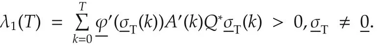
Following the simplification and reduction procedures adopted in the proof of Lemma 1 above for λ1(T),but now invoking the definition of the parameterin(12),we arrive at the inequalityEmploying this inequality in(a4),we conclude thatis positive ifwhich is the replacement in Corollary T1-1 for the condition[H-1]of Theorem 1.

Appendix 3 Proof of Lemma 3

We have,from(8)and(17),

Appendix 4 Proof of Lemma 4

Appendix 5 Proof of Lemma 5

Let the first part of the expanded version of the summation(35)be defined as

Based on condition[H-1]of Theorem 5 that ω(k)e−ξkA′(k)is non-increasing,we invoke the(discrete version of the)second mean value theorem:there is an index T′∈ [0,T]such that the right hand side of(a6)can be simplified to give

With the second part of the summation(35)defined by

and employing the condition of Theorem 5 that ω(k)eζkA′(k)is non-decreasing,we invoke the(discrete version of the)second mean value theorem,from which there is an index T′′∈ [0,T]such that the right hand side of(a8)can be simplified to give

We adopt the framework of the proof of Lemma 2 above,in the course of which we employ the parameters of(11)to reduce(a7)and(a9)to inequalities involving quadratic forms of,respectively,i)andand ii)andand combine the resultants with the reasoning adopted in[55,Pages 572–573],including the reference to condition[H-3](of Theorem 4),to conclude that λ5(T)of(35)is positive,if condition[H-2]of Theorem 5 is satisfied.

Appendix 6 Outline of proof of Lemma 6

Using(10)in(39),we get

With positive constants β1and β2chosen such that β1+β2=1,we consider its first part,viz.

where ξ is a nonnegative constant.Since ω(k)e−ξkA′(k)is nonincreasing by virtue of condition[H-1]of Theorem 6,by the second mean value theorem,there is an index T′∈ [0,T]for which(a11)can be written as

Concerning the last summation on the right hand side of(a12),letThen,invoking the definitions of CPs μi;(m,ℓ),μs;(m,ℓ)given in(13),we get the inequality

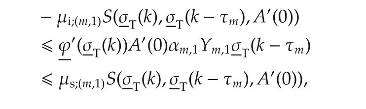
which,in combination with(a12),and withanddenoting,respectively,the positive and negative coefficients from the set{αm,ℓ(ℓ=1,2)},and under the assumption of the validity of interchange of the summation operations(with respect to k and m),leads to the inequality:

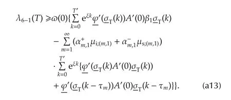
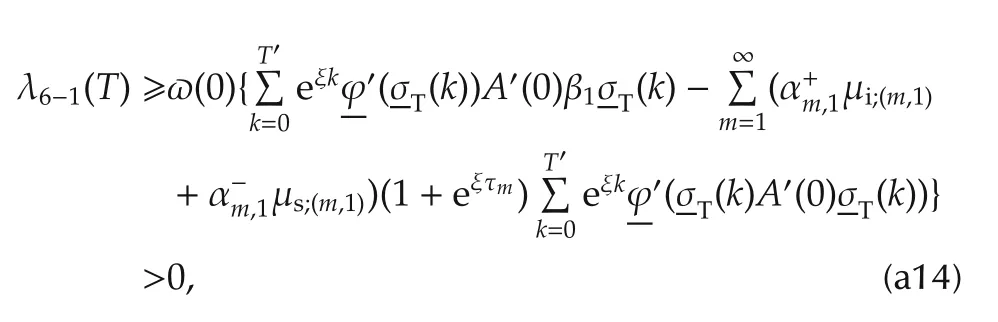
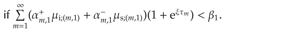
On the right hand side of(a13),in the second summation with respect to the(dummy)index k,involving the function of(k−τm),we can change the index k to k′≐ (k−τm),and revert to k after simplification,to get

We now consider the second part of the summation on right hand side of(a10).To this end,let

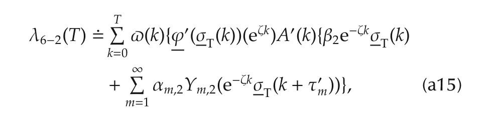
where ζ is a nonnegative constant.Since ω(k)eζkA′(k)is nondecreasing by virtue of condition[H-1]of Theorem 4,by the second mean value theorem,there is an index T”∈[0,T]for which(a15)can be written as

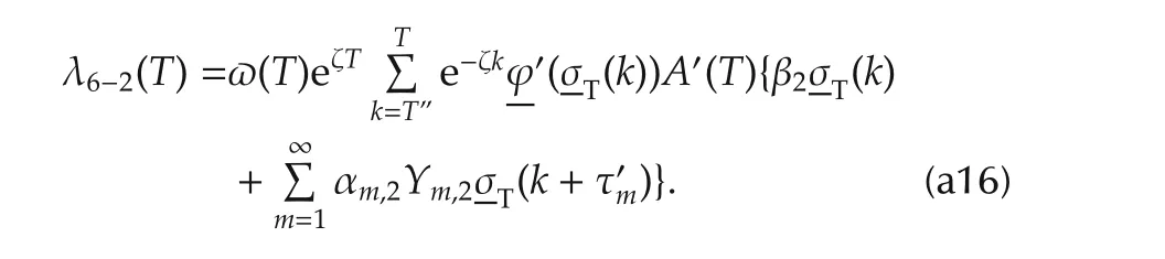
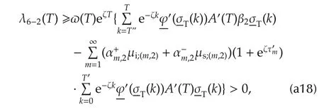
As before,concerning the last summation on the right hand side of(a16),letinvoking the definitions of CPsgiven in(13),we get the inequalitywhich,in combination with(a16),and withandefined as above,leads to the inequality:

On the right hand side of(a17),in the second summation with respect to the(dummy)index k,involving the function ofwe can change the index k toand revert to k after simplification,to get

Appendix 7 Outline of proof of Lemma 7

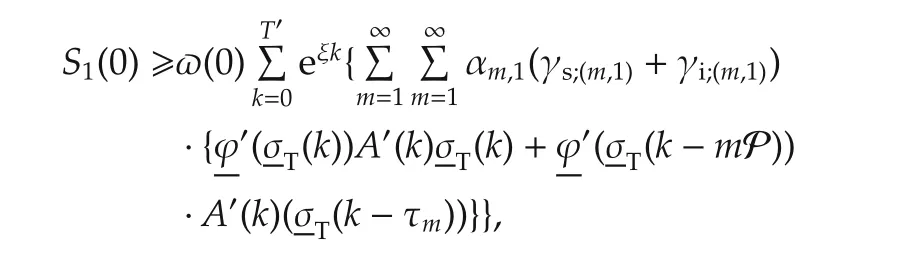
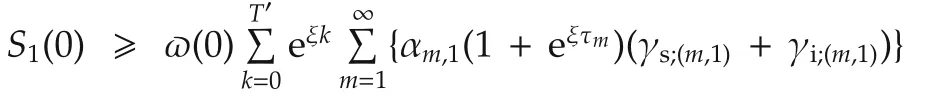
Our starting point is the set of equations(a10),(a11)and(a12)of the proof of Lemma 6.LetandFrom the monotonicity property(4)ofwe have

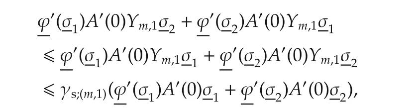
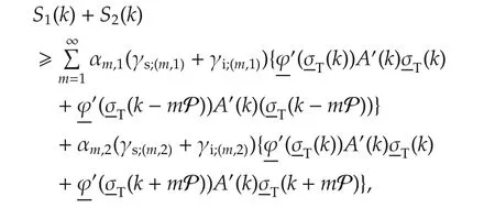
where γs;(m,1)is defined by(14),which we simplify to getwhere γi;(m,1)is defined by(14).Using the last inequality in the right hand side of S1(0)defined above,and noting that αm,1＜ 0,we get

Appendix 8 Other classes of nonlinearities and stability conditions

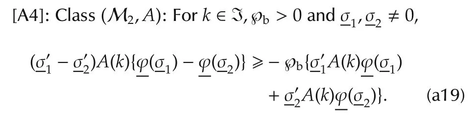
Piecewise(first-and-third-quadrant)nonlinearities having negative slopes also(but for which℘bcan be computed)are included in this class.Given ϕ(·)∈ (M2,A),its characteristic parameter℘bcan be obtained as a solution to a minimization problem:

If℘b= ∞,then(M2,A)becomes(N,A)for which no version of the generalized Popov-type matrix multiplier function can be employed even for a periodic A(k),without or with a restriction on the rate of variation of the elements of A(k).It has been found,however,that a generalized Popov-type matrix multiplier can be employed forwith a constraint on the rate of variation of the elements of A(k).This contrasts with the more general multiplier function meant for the class(M2,A)proposed in this paper.

[A5]:Class(N0,A):If there exists,a(scalar)potential function,such that,for k ∈ I,then(Alternatively,is conservative in the domain of definition of the vector function.This property guarantees the path-independence of line-integrals with respect to,involvingNote that the gradient operator∇is with respect to the components ofThe limits of the lineintegral used to define the class M3of nonlinearities later below involve only σ).

Note that,for an odd nonlinearity,V(·,σ)is even with respect toandA further sub-class of monotone functions corresponding to(M3,A)can be defined by inserting the right hand side expression of(a19)into the right hand side of(a21),before the equality sign.The CPis defined by(14).On the other hand,the CPs ofrecalling its property(a21),are defined by

Corollary T4-1Ifthen replace condition[H-1]of Theorem 3 bywhere℘bis defined by(a19).

The proof,which requires the use of the monotonicity property(a19)ofis similar to the proof of Lemma 4(based on the monotonicity property(4)).

Corollary L4-1Lemma 3 is valid forif condition[H-1]of Theorem 3 is replaced by the corresponding condition of Corollary T3-1.

CorollaryT4-2System(1)withandA(k)∈Cpis ℓ2-stable if,in Theorem 3,condition[H-1]is replaced by

Corollary L4-2Lemma 3 is valid forif condition[H-1]of Theorem 3 is replaced by the corresponding condition of Corollary T3-2.

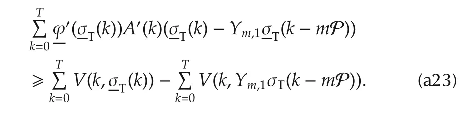
In the second summation of(a23),we change the index of summation k to τ =(k−mP),invoke the periodicity of V(k,·)and the properties of the summands with truncation,and simplify to conclude that

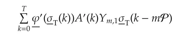
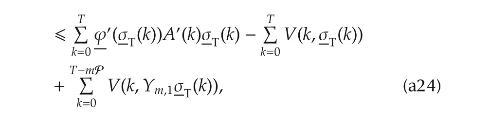
from which,invoking(a22),we conclude that the right hand side of(a24)can be replaced byMultiplying both the sides of the resultant inequality by αm,1＜ 0 for m=1,2,...,assuming the validity of an interchange of summation operations,and summing up,we get

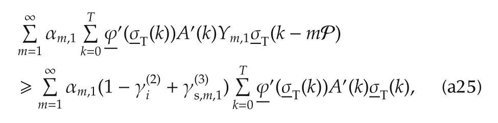
which we combine with the first summation on the right hand side of(a5)to conclude that

Corollary T7-1Ifthen replace[H-3]in Theorem 7 bywhere ℘bis defined by(a19).

Corollary T7-2Ifthen replace[H-3]in Theorem 7 bywhereandare defined by(a22).

Corollary L7-2Lemma 7 is valid for ϕ(·) ∈ (M3,K),if condition[H-1]of Theorem 7 is replaced by the corresponding condition of Corollary T7-2.

The proof of Corollary L7-2 is similar to that of Lemma 7.The starting point is the pair of equations(a12)and(a16),obtained by applying the condition[H-1]of Theorem 7(which is the same as the condition[H-1]of Theorem 6).For(a12),we invoke the assumption thatwith the governing inequality(a21),in which we identifywithandwithto get

In the second summation on the right-hand side of(a27),we change the(dummy)index of summation to τ =(k − τm),and invoke the properties of summands with truncation,and simplify to conclude that

from which,by invoking(a22),we conclude that the right hand side of(a28)can be replaced byMultiplying both the sides of the resultant inequality by αm,1＜ 0 for m=1,2,...assuming the validity of an interchange of the two summation operations,and summing up,we get

from which we conclude that

Y.V.VENKATESH(SM-IEEE’91)received the Ph.D.degree from the Indian Institute of Science(IISc),Bangalore,India.He was an Alexander von Humboldt Fellow at the Universities of Karlsruhe,Freiburg,and Erlangen,Germany;a National Research Council Fellow(USA)at the Goddard Space Flight Center,Greenbelt,MD;and a Visiting Professor at the Institut fuer Mathematik,Technische Universitat Graz,Austria,Institut fuer Signalverarbeitung,Kaiserslautern,Germany,National University of Singapore,Singapore and others.Apart from stability theory,his research interests include 3D computer and robotic vision;signal processing;pattern recognition;biometrics;hyperspectral image analysis;and neural networks.As a Professor at IISc,he was also the Dean of Engineering Faculty and,earlier,the Chairman of the Electrical Sciences Division.He is a Fellow of the Indian Academy of Sciences,the Indian National Science Academy,and the Indian Academy of Engineering.He is on the editorial board of the International Journal of Information Fusion.E-mail:yv.venkatesh@gmail.com.