Modeling tropical river runoff: A time dependent approach
Rashmi Nigam , Sudhir Nigam , Sushil K. Mittal
1. Dept. of Mathematics, University Institute of Technology, Rajiv Gandhi Technical University, Bhopal, India
2. Dept. of Civil Engineering, Lakshmi Narain College of Technology & Science, Bhopal, India
3. Dept. of Civil Engineering, Maulana Azad National Institute of Technology, Bhopal, India
1 Introduction
Rainfall and runoff are highly non-linear and complex outcomes of nature which require sophisticated data analysis for accurate modeling and simulation. Rainfall and runoff modeling is of particular relevance for engineering applications of water as well as in flood disaster management. Flood forecast modeling specifies the trends of river level (rising or falling) and the quantum of runoff (low/medium/high) to assess the likely loss of property and life (Singh and Woolhiser, 2002).
Simulation of river runoff series over time is an essential part for real time quantification of water for planning and management of water resource systems. Real time flood forecasting is an effective non-structural methodology for flood management. Flood estimates can be calculated well in advance to provide sufficient lead time for authorities to implement flood management strategies. The stochastic time series modeling approach can be used to characterize and predict river runoff of a nonperiodic and chaotic nature.
This paper aims to describe an accurate modeling method to forecast the runoff of the Kulfo River, which flows through the southern part of Ethiopia. The water in this river is mainly utilized for irrigation and water supply for public consumption. Advance estimation of the volume of river runoff can be effectively utilized to plan irrigation schemes and water supply projects. This study of the forecasting models developed using historical runoff data of different durations will lead to better selection criteria for planning optimal water supplies.
2 Background
In the past, time series studies of rainfall runoff processes consisted of syntheses of available annual hydro-logic data in time-dependent or independent stochastic components, and subsequent identification of trends and cycles (Matalas, 1963; Yevjevich, 1972). The simplest time series model, which deals with one only type of data,has three components to describe the linear stochastic process: autoregression (AR), integration (I) and moving average (MA) which can be combined as the autoregressive integrated moving average (ARIMA) model (Box and Jenkins, 1970). Various other linear and dynamic regression derivatives of the ARIMA process, including PARIMA, SARIMA, DARIMA, ARMAX, NRL, MLR,and VARMA were developed over the years (McKerchar and Delleur, 1974; Hipelet al., 1977; Salaset al., 1980;Changet al., 1984; Haltiner and Salas, 1988; Wang,2006). These models have long been applied in the modeling of rainfall runoff and forecasting stream flows and floods (Noakeset al., 1985; Salas, 1992; Bender and Simonovic, 1994; Maríaet al., 2004).
Graupeet al. (1976) used the ARIMA model for simulating water flow in karstic basins. Kumar (1980)and O’Connell (1980) used time series to forecast flood episodes consequent to rainfall occurrence. Chang and Tiao (1985) and Weeks and Boughton (1987) attempted to create an accurate flood forecast system using time series methods. Chiewet al. (1993), Clapset al. (1993), and Cheng (1994) used ARIMA to forecast rainfall runoff at different catchments of varying scales. Maidment (1993)suggested use of the periodic autoregressive (PAR), periodic autoregressive moving average (PARMA) and periodic gamma autoregressive (PGAR) models for single and multiple periodic time series. Broersen (2008) developed the time series analysis software ARMASA.
Hsuet al. (1995) compared the ARIMA method with artificial neural network modeling, followed by Zhang and Govindaraju (2000), Young (2002), Cigizoglu (2003),Sanaet al. (2003), Organ and Yalcin (2004), Kisi (2005),and DeSilva (2006), who attempted time series analysis with the inclusion of nonlinear mathematical approaches and artificial intelligence methods of forecasting. Wanget al. (2008), Naill and Momani (2009), and Volkan and Onkur (2010) have studied mixed time series models coupled with other models to devise new approaches.
The selection of the modeling and forecasting method used in this work was based upon the hydraulic characteristics of river flow and runoff events (which are highly influenced by the previous stages of river inflow). Our assessment of the study of the above cited literatures led us to conclude that ARIMA time series modeling may yield reliable and better forecasts (flow estimation) for the perennial Kulfo River and we therefore applied the ARIMA time series modeling approach to forecast runoff of this River.
3 Study area
The Kulfo River is a perennial medium-sized hilly river that originates in the highlands and ridges of Haringa, Kecha and Tiba (names of areas surrounding the river) in the southern part of Ethiopia. The river runs along the border of the Great Rift Valley and spans the great Abaya-Chamo lake basin. The river catchment area is about 16,400 km2. Figure 1 shows the geographical coordinates defining the boundaries of the river catchment, the general terrain type, and the water course of the Kulfo River, which has a total drainage area of about 492 km2.
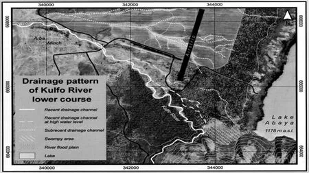
Figure 1 Drainage pattern of catchment area of the Kulfo River (Source: Schutt and Thiemann, 2006)
The elevation of the catchment varies from 1,108 to 3,600 m a.s.l.. This river joins the outflow from the Abaya and the flow from Arba Minch ("Forty Springs") to enter Chamo Lake. The current study site lies at the lower reach of the Kulfo River near the town of Arba Minch where the length of the river is about 4,570 m, and the main tributaries forming the Kulfo River are the Titika and the Gulando. A stream called the Yermo joins the Kulfo River, to flow through the lower portion of the river. The mean annual flow (at upper hydrological station) is 4.66 m3/s; after fusion, the outflow of the Abaya runoff increases to 13.49 m3/s.
In this study we used rainfall data that was recorded at the Arba Minch meteorological station situated close to Abhaya Lake and about 1 km away from the Kulfo River bank. The rainfall pattern (as shown in figure 1) is mostly indefinite but it frequently inundates the Kulfo River Basin. Depending upon the distribution of rainfall intensity the river has a response time of about six to eight hours for the runoff to set.
4 Methodology
In this study the forecasts of mean monthly runoff from the Kulfo River using 10-year and 20-year data(1977–1987 and 1977–1997) are compared. Our analysis of rainfall and runoff data of the Kulfo River was carried out in the following stages:
· Statistical analysis
· Data preprocessing
· Model selection and development
· Generation of model forecasts
· Residual analysis
· Evaluation of model forecasts
We performed descriptive statistical analyses of the rainfall and runoff data of the Kulfo River to elucidate the patterns and trends in the data over time. The details of the descriptive attributes are readily available in statistics literature, including Rashmi (2012).
Data preprocessing is part of the ARIMA model development process whereby trends, seasonality, cyclic patterns and stationarity of the data are recognized by means of visiual inference derived from the time-variant plots of rainfall and runoff data, regression analyses,moving averages and differencing of the data (Box and Jenkins, 1970; Vandaele, 1983).
Vandaele (1983) described a univariate ARIMA model, which has an integrating attribute of a time series.One shorthand notation for this model (having a seasonality component) is ARIMA (p,d,q) × (P,D,Q)s, wheresdenotes the seasonality term. If the preliminary analysis and preprocessing uncover seasonal variations in the data,the ARIMA equation is reduced to ARIMA (p,d,q)which can be expressed by the following general equation:

A structural expansion of the non-seasonal equation is:

whereytis the stationary series after differencing (1-B)dYt;Ytis the input variable with reference to time;dis the number of nonseasonal differencing;Bis the backward shift operator, defined asBy=yt-1;pis the order of an autoregressive term used in the autocorrelation function (ACF) plot;qis the order of a moving average term used in the partial autocorrelation function (PACF)graphs; andφandθare the nonseasonal parameters of the AR (p) and MA (q) order, respectively.
In cases where the rainfall or runoff data show a non-stationary pattern, the data series need to be converted into a stationary time series by means of differencing, using the backward shift operator as defined in the terms of the above equations. The first values of AR(p) and MA (q) are estimated through the moments(Yule-Walker equations) (Box and Jenkins, 1970), and their subsequent estimations are done using the iteration process via the maximum likelihood method. Residuals’checking is done to verify the adequacy of the fitted model by testing the residuals of the fitted series. The ACF and PACF of the residual series are plotted and are checked for 95% significance. In a best-fit model, there is no inherent meaning in the residuals pattern. The values of ACF and PACF dies off within the 95% significance line indicating almost zero noise in the residual series(Section 5.5 below).
Models can be confirmed or evaluated by the demonstration of good agreement between several sets of observations and predictions. Performance measures and efficiency criteria are used to evaluate "how well a model simulation fits the available observations" (Beven, 2001).Our study used the following measures to judge the performance of the stochastic model:
· Coefficient of correlation (CC)
· Coefficient of determination (CD)
· Nash-Sutcliffe efficiency (E)
· Index of agreement (d)
· Relative efficiency criteria (Ereland drel)
· Fractional bias (FB)
Most of the efficiency criteria contain a summation of the error term (the difference between the simulated and the observed variable at each time step) normalized by a measure of the variability in the observations. We computed the following errors to assess the model’s capabilities:
· Mean bias error (MBE)
· Mean absolute error (MAE)
· Root mean square error (RMSE)
· Normalized mean square error (NMSE)
Detailed descriptions and formulae of the above statistical measures and errors can be found in Rashmi(2012) and Nigamet al.(2013).
The increased data strength not only supports a parsimonious model but also presents features to validate results of model when applied on short or discontinuous time series (Clapset al., 1993). Therefore, in this study two ARIMA models were developed to forecast river runoff based upon 10-year and 20-year data to determine the impact of the lengthened data set on the forecast efficiency.
5 Results and discussion
Our runoff forecasting model for the Kulfo River was developed in the following stages:
5.1 Statistical analysis
The average monthly rainfall and runoff data of the Kulfo River (1977–1996) are plotted in figure 2. As shown in the figure the variation in runoff quantity is dependent upon the rainfall. The relatively higher runoff during the years 1987–1988 and 1991–1994 was an obvious result of greater annual rainfall in those time periods. The sudden rise in runoff was due to excessive rainfalls.
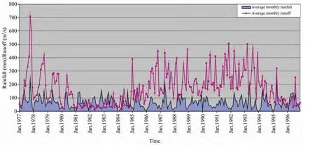
Figure 2 Average monthly rainfall and runoff of the Kulfo River
The histogram and normal frequency distribution curves of river runoff for the years 1977–1986 and 1977–1996 are shown in figure 3. Clearly, the runoff frequency distribution graph in 20 years (1977–1996)showed more non-normal deviation and there were more extreme runoff events than low-runoff episodes. The area inside the normal curve, which indicates the runoff volume is larger in the 20 years span.
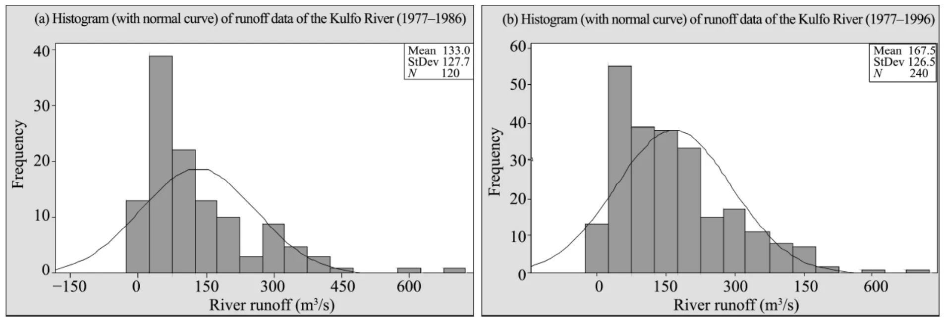
Figure 3 Histogram and frequency distribution of runoff
The descriptive statistics of the river runoff data are presented in table 1. There is vast variation in the minimum and maximum runoff values. The mean runoff is about 50% higher in the 20 years period. Comparison of the mean and median values indicates a total shift of the data toward the lower end of the mean. The coefficient of variation measures the variability relative to the mean.The standard deviation indicates the dispersion of runoff values from the mean. In the 20-year runoff data, the nearly equal values of the standard deviation and the lower values of the standard error of mean (SE Mean)indicate a precise estimation of the data. Small values of skewness and kurtosis show that the 20-year runoff values are robust and centralized toward the mean.
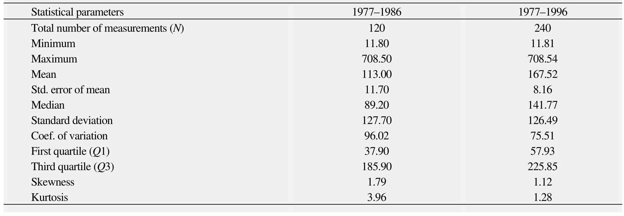
Table 1 Descriptive statistics of runoff data
Box plots of the 10-year and 20-year data (Figure 4)show that the distribution of the runoff data is generally centered on the mean values. The very extreme runoffs occurred only in the first decade. The box plots also display outlier observations beyond the upper or lower whiskers (extent of boundaries).
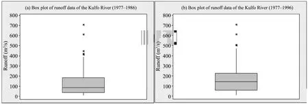
Figure 4 Box plots of runoff data of the Kulfo River
The individual value plots of runoff data of the Kulfo River (Figure 5) shows when the river runoff was available continuously and also when it declined. It is clear that there were more outlier runoff events in the 10-year duration, although the mean level of river runoff increased during the 20-year span.
5.2 Data preprocessing
In tropical regions, rainfall and runoff processes are more cyclic than seasonal. ARIMA can be used to model patterns that may not be visible in plotted data. For identification of the parsimony order of the ARIMA model parameters (p,d,q,P,D,Qands), we plotted the autocorrelation function (ACF) and partial autocoreelation function (PACF) of the 10-year and 20-year runoff time series for various combinations of differencing (d=0andd=1) and lags (N/4,Nbeing the number of observations). The selected graphs are given in figures 6 and 7 respectively.
5.3 Model selection and development
From inspection of the ACF and PACF, the parsimony orders of the ARIMA model were ARIMA (1, 1, 1)and ARIMA (1, 0, 1) for the runoff data of 10 years(1977–1986) and 20 years (1977–1996), respectively.The identified parameters were then evaluated to develop our forecasts, using the following equations:
For the ARIMA (1, 1, 1) process:

For the ARIMA (1, 0, 1) process:

where the terms are as defined in equation(1).
5.4 Generation of model forecasts
Runoff forecasts were generated from both models.Forecasts were generated for one year (1987) from the model ARIMA (1, 1, 1) and for another year (1997) from the model ARIMA (1, 0, 1). These forecasts are plotted with actual river runoff in figure 8 and figure 9 respectively. The forecast graphs well capture the trends and patterns of the runoff. Clearly the forecasts in the ARIMA (1, 1, 1) model are under predictive, whereas in the ARIMA (1, 0, 1) model the forecasts are mostly overpredictive and the gaps in quantification of runoff during high flows are larger. Thus both models well capture the runoff trends during high runoffs but the ARIMA(1, 0, 1) model falls fails to provide satisfactory estimation of flow during both high flows and low flows. This may be attributed to our exclusion of non stationarity.
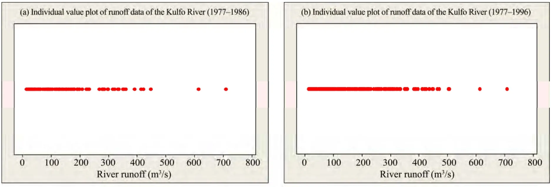
Figure 5 Individual value plots of river runoff

Figure 6 Autocorrelation function of river runoff

Figure 7 Partial autocorrelation function of river runoff
The ARIMA (1, 0, 1) model is bungling to meet up the extreme runoff episodes and beside the overpredictive nature it behaves diminutive for high flows thus targeting towards a mean flow sympathy. The forecasting error clearly decreases with the reducing runoff values, and the quantitative forecasting estimate given by both models are reasonably accurate when the runoff values are in the moderate range.
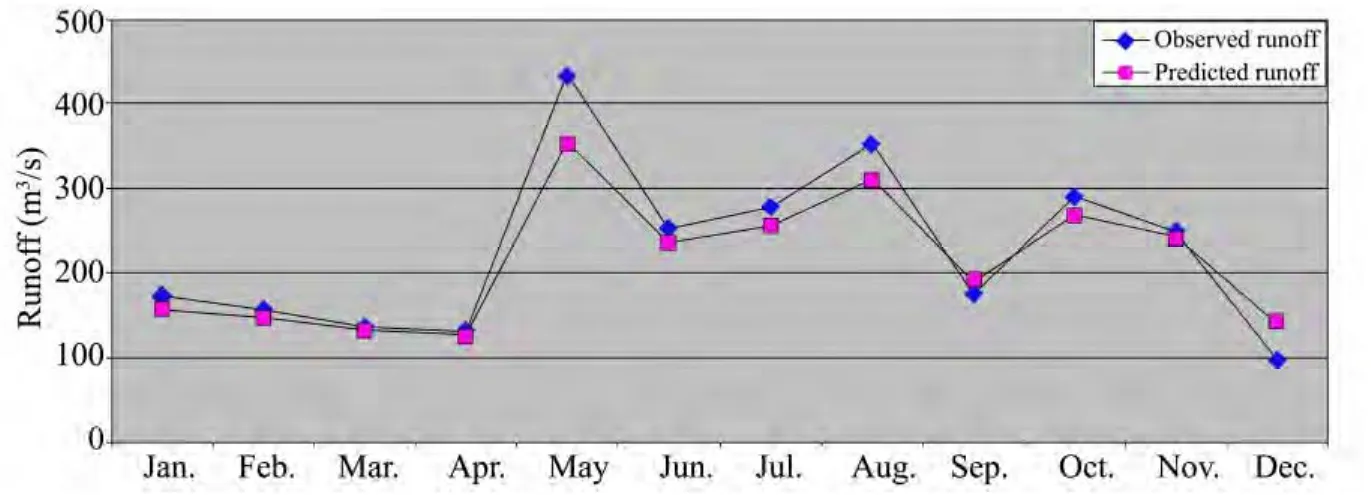
Figure 8 Observed vs. predicted runoff of the Kulfo River during 1987 using ARIMA (1, 1, 1) model
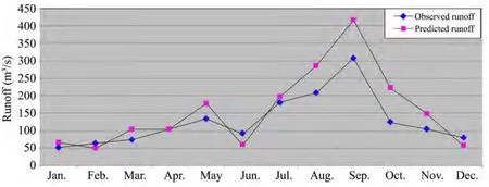
Figure 9 Observed vs. predicted runoff of the Kulfo River during 1997 using ARIMA (1, 0, 1) model
5.5 Residual analysis
To determine the goodness of fit of both models, we assessed the values of ACF and PACF. The desirable outcome would be that these values exihibit a random pattern floating on either sides of 0 (a non-random pattern would violate the assumption that the predictor variables are unrelated to the residuals). We worked out the residuals for the model validation and to check for the existence of any noise. We plotted the ACF and PACF of the residuals to see whether a pattern exceeds the 5% confidence limits in the fitted models (Figures 10 and 11).From the ACF and PACF residual graphs of both the ARIMA (1, 1, 1) and ARIMA (1, 0, 1) models, which both generally trend toward negligible to zero, it is clear that the selected models are parsimonious and have good fits. Thus, the residual analyses indicate that these model forecasts meet the requirement of a perfect fit model, but the ARIMA (1, 0, 1) model is strongly recommended for long term predictions of mean monthly runoff of the Kulfo River since an overpredictive model is always better than an underpredictive model (e.g., ARIMA (1, 1, 1)in our study) in view of flood management and safety of subsequent losses.

Figure 10 ACF of the residuals of the 10-year and 20-year model forecasts

Figure 11 PACF of the residuals of the 10-year and 20-year model forecasts
5.6 Evaluation of the model forecasts
Precise evaluation of models of natural systems is very difficult, because natural systems are never closed, whereas model solutions are always non-unique. Thus there is usually an unresolved problem of linking field measurements with the model predictions due to heterogeneity, scale effects, nonlinearities or measurement techniques. The random nature of the process also leads to a certain irreducible inherent uncertainty. Thus models can only be confirmed or evaluated by the demonstration of good agreement between several sets of observations and predictions.We computed various statistical measures and errors(Table 2) to determine the runoff forecasting efficiency of the fitted models ARIMA (1, 1, 1) and ARIMA(1, 0, 1). We then compared the numerical values of the evaluation parameters with the standard values to ascertain the validity, accuracy, and efficiency of the model forecasts.
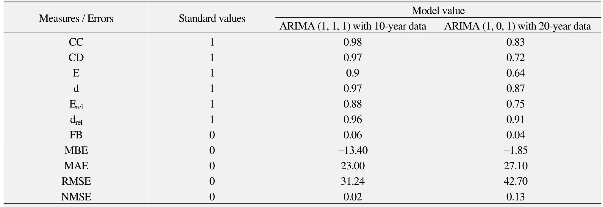
Table 2 Performance measures and errors
From the table 2, it is clear that the ARIMA (1, 1, 1)model with 10-year data performs better than the ARIMA (1, 0, 1) model based upon 20-year of runoff data. However, the nature of the errors and their extents are reasonably similar for both models.
6 Conclusion
Time series plots of historical rainfall and runoff data of the Kulfo River in Ethiopia indicate that the river runoff rapidly rises when there is precipitation, and quickly decreases after the rain ends, but the river runoff continues to diminish for a long time after the precipitation ends because of contribution from river base-flow.Our forecast graphs (Figures 8 and 9) well capture the trends of runoff, and quantitative predictions of runoff can be made from both graphs (models) in terms of average runoff values. Although the forecast graphs are insensitive to extreme variations in runoff, the ARIMA models we developed are able to nicely capture the high runoff peaks resulting from abrupt rainfalls over the catchment area and the Kulfo River tributaries.
The ARIMA process is appropriate for modeling the linear and uniform patterns of runoff but falls short in simulating the non-linear, non-uniform and complex aspects of runoff. Due to the highly variable nature of runoff, a parsimonious model could not always provide best-fit forecasts for an entire span of data. In most practical cases, insufficient data prevent the use of a parsimonious, powerful, but demanding model. Nevertheless, an ARIMA model can include both the high and low values of runoff and their vacillations to provide a reasonable quantification of runoff during odd or unusual river flow circumstances, and these models could be exploited to predict upcoming abrupt changes in runoff conditions.
The ARIMA (1, 0, 1) model based upon 20-year data, which is more parsimonous than the ARIMA (1, 1,1) model based upon 10-year data, proved to be deficient in forecasting peak runoffs. This is contrary to the general consensus that a parsimonious model always gives better results. The reason why this parsimonious model failed to produce better runoff predictions lies in the nonlinear nature of the data. Fitted ARIMA models perform better for runoff simulation when the mean levels have fewer irregular and sharp nodes. This clearly indicates that the performance of ARIMA model is mainly governed by the distributive properties of the data rather than the length of the data acquisition period.A well distributed (normal) dataset usually shows better modeling and simulation efficiencies. However, the forecast efficiency can be improved by use of higher resulation data. Based upon these consideration ARIMA(1, 1, 1) model based on 10-year data is recommended for the estimation of future river water quantities and advance warning of floods.
Bender M, Simonovic S, 1994. Time-series modeling for long-range stream-flow forecasting. Journal of Water Resources Planning and Management, 120(6): 857–870.
Beven JK, 2001. Rainfall-Runoff Modelling––The Primer. John Wiley& Sons Ltd., pp. 319.
Box GEP, Jenkins GM, 1970. Time Series Analysis: Forecasting and Control. Holden-Day, San Francisco.
Broersen PMT, 2008. Time series models for spectral analysis of irregular data far beyond the mean data rate. Meas. Sci. Technol., 19(1):015103. DOI: 10.1088/0957-0233/19/1/015103.
Chang LC, Tiao J, 1985. Microcomputer application in stochastic hydrology. Conference Proceedings of Hydraulics and Hydrology in the Small Computer Age, American Society of Civil Engineers,Reston, VA, pp. 371–375.
Chang LC, Tiao J, Kavas ML,et al., 1984. Daily precipitation modeling by discrete ARMA processes. Journal of Water Resources Research, 20(5): 565–580. DOI: 10.1029/WR020i005p00565.
Cheng Y, 1994. Evaluating an autoregressive model for stream flow forecasting. Conference Proceedings of Hydraulic Engineering, pp.1105–1109.
Chiew FHS, Stewardson MJ, McMahon TA, 1993. Comparison of six rainfall-runoff modelling approaches. Journal of Hydrology, 147:1–36. DOI: 10.1016/0022-1694(93)90073-I.
Cigizoglu HK, 2003. Incorporation of ARMA models into flow forecasting by artificial neural networks. Environmetrics, 14(4):417–427. DOI: 10.1002/env.596.
Claps P, Rossi F, Vitale C, 1993. Conceptual stochastic modeling of seasonal runoff using ARMA models and different time scales of aggregation. Water Resource Research, 29(8): 2545–2559.
DeSilva MAP, 2006. A time series model to predict the runoff of catchment of the Kalu Ganga Basin. Journal of National Science Foundation, Sri Lanka, 34(2): 103–105. DOI:10.4038/jnsfsr.v34i2.2089.
Graupe D, Isailovic D, Yevjevich V, 1976. Prediction model for runoff from karstified catchments. Proceedings of the U.S.-Yugoslavian Symposium on Karst Hydrology and Water Resources, Dubrovnik,June 2–7, 1975, pp. 277–300.
Haltiner JP, Salas JD, 1988. Short-term forecasting of snowmelt discharge using ARMAX model. Journal of the American Water Resources Association, 24(5): 1083–1089.
Hipel KW, Mcleod AI, Lennox WC, 1977. Advances in Box-Jenkins modeling. Journal of Water Resource Research, 13(3): 567–575.DOI: 10.1029/WR013i003p00567.
Hsu K, Gupta HV, Sorooshian S, 1995. Artificial neural network modeling of the rainfall––runoff process. Journal of Water Resources Research, 31(10): 2517–2530. DOI: 10.1029/95WR01955.
Kisi O, 2005. Daily river flow forecasting using ANN and autoregressive models. Turkish Journal of Engineering and Environmental Sciences, 29(1): 9–20.
Kumar A, 1980. Prediction and real-time hydrological forecasting. Ph.D.dissertation, Indian Institute of Technology, Delhi, India.
Maidment DR, 1993. Handbook of Hydrology. McGraw-Hill, New York.
María CM, Wenceslao GM, Manuel FB,et al., 2004. Modeling of the monthly and 13 daily behaviour of the discharge of the Xallas River using Box–Jenkins and N networks methods. Journal of Hydrology,296: 38–58.
Matalas NC, 1963. Autocorrelation of rainfall and stream flow minimums.In: Geological Survey, Professional Paper, Statistical Studies in Hydrology, Government Printing Office, Washington D.C., pp. 434.
McKerchar AI, Delleur JW, 1974. Application of seasonal parametric linear stochastic model to monthly flow data. Journal of Water Resources Research, 10(2): 246–255. DOI:10.1029/WR010i002p00246.
Naill PE, Momani M, 2009. Time series analysis model for rainfall data in Jordan: Case study. American Journal of Environmental Sciences,5(5): 599–604. DOI: 10.3844/ajessp.2009.599.604.
Nigam R, Nigam S, Kapoor S, 2013. Time series modeling of tropical river runoff. International Journal of Pure and Applied Research in Engineering & Technology, 1(7): 13–29.
Noakes DJ, McLeod AI, Hipel KW, 1985. Forecasting monthly river flow time series. International Journal of Forecasting, 1(2):179–190.
O’Connell PE, 1980. Real-Time Hydrological Forecasting and Control.Oxfordshire, Institute of Hydrology, UK, pp. 264–295.
Organ D, Yalcin A, 2004. Flood Forecasting Using Nonlinear Time Series Analysis. REU Report, University of South Florida, College of Engineering, Tampa, FL.
Rashmi N, 2012. Development of computational modeling framework for river flow forecasting. Ph.D. dissertation, Dept. of Mathematics, Maulana Azad National Institute of Technology,Bhopal.
Salas JD, 1992. Analysis and modeling of hydrologic time series. In:Maidment DR (ed.). Handbook of Hydrology, McGraw-Hill, New York, pp. 19.1–19.72.
Salas JD, Deulleur JW, Yevjevich V,et al., 1980. Applied Modelling of Hydrologic Time Series. Water Resources Publications, Littleton, CO.
Sana BH, Nejib S, Mahmoud G,et al., 2003. The Box-Jenkins analysis and neural network: prediction and time series modeling. Applied Mathematical Modeling, 27: 805–815.
Schutt B, Thiemann S, 2006. Kulfo River, south Ethiopia as the regulator of lake level change in the Lake Abaya-Lake Chamo system.Zentralblatt für Geologie und Paläontologie, Teil 1/2, Stuttgart,Marz, pp. 29–143.
Singh VP, Woolhiser DA, 2002. Mathematical modeling of watershed hydrology. Journal of Hydrology Engineering, 7(4): 270–292.
Vandaele W, 1983. Applied Time Series and Box-Jenkins Models.Academic Press, New York.
Volkan B, Onkur A, 2010. A Study on Modeling Daily Mean Flow with MLR, ARIMA and RBFNN. BALWOIS 2010, Ohrid, Rep. of Macedonia, pp. 25.
Wang W, 2006. Sochasticity, Nonlinearity and Forecasting of Streamflow Processes. IOS Press, Technical University of Delft, The Netherlands.
Wang YC, Chen ST, Yu PS,et al., 2008. Storm-even rainfall-runoff modelling approach for ungauged sites in Taiwan. Hydrological Processes, 22(21): 4322–4330. DOI: 10.1002/hyp.7019.
Weeks WD, Boughton WC, 1987. Tests of ARMA Model forms for rainfall-runoff modeling. Journal of Hydrology, 91(1–2): 29–47.DOI: 10.1016/0022-1694(87)90126-0.
Yevjevich VM, 1972. Stochastic Processes in Hydrology. Water Resource Pub., FC, Colorado.
Young PC, 2002. Advances in real-time flood forecasting. Philosophical Transactions of the Royal Society, 360: 1433–1450. DOI:10.1098/rsta.2002.1008.
Zhang B, Govindaraju RS, 2000. Prediction of watershed runoff using Bayesian concepts and modular neural networks. Journal of Water Resources Research, 36(3): 753–762. DOI:10.1029/1999WR900264.
 Sciences in Cold and Arid Regions2014年3期
- Sciences in Cold and Arid Regions的其它文章
- Spatiotemporal variations of maximum seasonal freeze depth in 1950s–2007 over the Heihe River Basin,Northwest China
- Retrieval study of lake water depth by using multi-spectral remote sensing in Bangong Co Lake
- Climate transformation to warm-humid and its effect on river runoff in the source region of the Yellow River
- Water sources of plants and groundwater in typical ecosystems in the lower reaches of the Heihe River Basin
- Effects of fertilization on population density and productivity of herbaceous plants in desert steppe
- Effects of sand burial on dune plants: a review
