Numerical modeling of flow in continuous bends from Daliushu to Shapotou in Yellow River

He-fang JING, Chun-guang LI*, Ya-kun GUO, Li-jun ZHU, Yi-tian LI

1. School of Civil Engineering, Beifang University of Nationalities, Yinchuan 750021, P. R. China

2. School of Engineering, University of Aberdeen, Aberdeen AB24 3UE, UK

3. School of Mathematics and Information Science, Beifang University of Nationalities, Yinchuan 750021, P. R. China

4. State Key Laboratory of Water Resources and Hydropower Engineering Science, Wuhan University, Wuhan 430072, P. R. China

Numerical modeling of flow in continuous bends from Daliushu to Shapotou in Yellow River

He-fang JING1, Chun-guang LI*1, Ya-kun GUO2, Li-jun ZHU3, Yi-tian LI4

1. School of Civil Engineering, Beifang University of Nationalities, Yinchuan 750021, P. R. China

2. School of Engineering, University of Aberdeen, Aberdeen AB24 3UE, UK

3. School of Mathematics and Information Science, Beifang University of Nationalities, Yinchuan 750021, P. R. China

4. State Key Laboratory of Water Resources and Hydropower Engineering Science, Wuhan University, Wuhan 430072, P. R. China

The upper reach of the Yellow River from Daliushu to Shapotou consists of five bends and has complex topography. A two-dimensional Re-Normalisation Group (RNG) k-ε model was developed to simulate the flow in the reach. In order to take the circulation currents in the bends into account, the momentum equations were improved by adding an additional source term. Comparison of the numerical simulation with field measurements indicates that the improved two-dimensional depth-averaged RNG k-ε model can improve the accuracy of the numerical simulation. A rapid adaptive algorithm was constructed, which can automatically adjust Manning’s roughness coefficient in different parts of the study river reach. As a result, not only can the trial computation time be significantly shortened, but the accuracy of the numerical simulation can also be greatly improved. Comparison of the simulated and measured water surface slopes for four typical cases shows that the longitudinal and transverse slopes of the water surface increase with the average velocity upstream. In addition, comparison was made between the positions of the talweg and the main streamline, which coincide for most of the study river reach. However, deviations between the positions of the talweg and the main streamline were found at the junction of two bends, at the position where the river width suddenly decreases or increases.

numerical simulation; RNG k-ε model; Yellow River; continuous bend; circulation flow; adaptive algorithm regarding Manning’s roughness coefficient

1 Introduction

Flow in almost all natural rivers is turbulent and complicated, especially in rivers with bends and complex topography. Accurate simulation of flow in natural rivers can only be achieved using turbulence closure models. Many turbulence closure models have beendeveloped, such as the zero equation model, k-ε model, Reynolds stress model (RSM), and algebraic stress model (ASM) (Versteeg and Malalasekera 1995). The zero equation model is the simplest of all turbulence models, but it depends on some empirical coefficients, which limits its application. The RSM and the ASM can be used to simulate complex flow in meandering open channels (Sugiyama et al. 2006; Jing et al. 2009, 2011). However, these models are more complicated and require more computational time than other models. This limits their application in simulating natural river flow. The k-ε model has a high degree of versatility and needs less computation time than the RSM and the ASM. As a result, it is widely used to numerically simulate all kinds of flows, such as open-channel flows, river flows and pipe flows (Humphery and Pourahmadi 1983; Amano et al. 1984; Guo et al. 2007, 2008).

However, the standard k-ε model may produce distorted results when it is used to simulate some complex flows, such as flow with a high strain rate and flow with a large streamline curvature (Pezzinga 1994). For flow with a high strain rate and a large streamline curvature, the Re-Normalisation Group (RNG) k-ε model, an improvement of the standard k-ε model, should be used in order to obtain accurate simulation results (Speziale and Thangam 1992).

When the computational domain is very large, three-dimensional (3D) numerical simulation is very time consuming. Therefore, 3D mathematical models are usually averaged in the depth direction, and two-dimensional (2D) depth-averaged mathematical models are produced. Generally speaking, 2D depth-averaged models cannot reflect the influence of circulation flow in rivers with bends. Thus, the simulated results are usually not satisfactory in rivers with bends. In order to solve this problem, various schemes have been presented in recent years. Molls and Chaudhry (1995) proposed the concept of integrated effective stress, including laminar viscosity stress, turbulent stress, and dispersion stress due to depth averaging, but they ignored the nonuniform distribution of vertical velocity in a bend flow simulation. Nagata et al. (1997) presented a 2D depth-averaged model in which the secondary flow component was derived using the vertical distribution of main and transverse velocities. Lien et al. (1999) proposed a 2D depth-averaged model that takes into account the influence of secondary flow through calculation of the dispersion stress produced by the discrepancy between the mean and true velocity distributions. However, the process of calculating the additional source term in the model is very complicated. Furthermore, the governing equations are presented in the orthogonal curvilinear coordinates and the velocity components are not original ones in the x and y directions. Kimura et al. (2010) used a 2D depth-averaged model to simulate open-channel flow with a side cavity, in which the effects of secondary currents are integrated by adding an extra source term in the momentum equations. However, it can only be used in laboratory regular bend channels.

In the numerical simulations of open-channel and river flows, Manning’s roughness coefficient plays an important role. The selection of Manning’s roughness coefficient can lead to the success or failure of the whole numerical simulation. In practical application, the valueof Manning’s roughness coefficient usually varies in the computational domain (Guo et al. 2012). The usual approach to setting the value of Manning’s roughness coefficient in numerical simulation is to choose an estimated value based on experience. The value is then adjusted in the simulation according to numerical results until the numerical results agree with the measured data. Each time the Manning’s roughness coefficient is modified, the whole program needs to be run once more. Usually, this process is very time consuming, especially when the value of Manning’s roughness coefficient varies in the computational domain.

In this study, a 2D depth-averaged RNG k-ε model was developed by depth-averaging the 3D RNG k-ε model, and it was improved by adding an extra source term in the momentum equations in a body-fitted coordinate system. Numerical examples indicate that the improved 2D depth-averaged RNG k-ε model can reasonably simulate the turbulent flow in rivers with continuous bends.

An adaptive algorithm was developed to automatically search for the appropriate value of Manning’s roughness coefficient in the computational domain, which can save a lot of trial computational time. The improved 2D depth-averaged RNG k-ε model was used to investigate the hydraulic elements in the Daliushu-Shapotou Reach of the Yellow River. The simulated velocity and water level agree with the field-measured data. Water surface slopes were simulated in four cases and analyzed. In addition, consistency between the positions of the talweg and main streamline was investigated.

2 Mathematical model

2.1 2D depth-averaged RNG k-ε model in Cartesian coordinates

The 2D depth-averaged RNG k-ε model in Cartesian coordinates includes the following equations (Versteeg and Malalasekera 1995; Wu et al. 2003):

The continuity equation:

The momentum equation in the x direction:

The momentum equation in the y direction:

The k-equation:

The ε-equation:

where z is the water level; h is the water depth; u is the vertically averaged velocity in the x direction; v is the vertically averaged velocity in the y direction; t is time; ν is the kinematic viscosity of water; νtisthe eddy viscosity coefficient of water, where νt= Cμk2ε, with Cμbeing a constant; k is the turbulent kinetic energy; ε is the turbulence dissipation rate; g is the acceleration of gravity; n is Manning’s roughness coefficient; αkand αεare constants; and Skand Sεare the source terms in the k-equation and ε-equation, respectively, which can be calculated as follows:

The constants and their values in the model are shown in Table 1 (Yakhot and Orzag 1986).

Table 1 Values of constants in 2D depth-averaged RNG k-ε model

2.2 Improved 2D depth-averaged RNG k-ε model

As the study river consists of several irregular bends where strong circulation flow exists, the 2D depth-averaged RNG k-ε model usually cannot reflect the influence of such flow. In this case, the model needs to be modified to take the influence of circulation flow into account.

The Poisson equation method (Versteeg and Malalasekera 1995) was used to convert the governing equations in Cartesian coordinates into body-fitted coordinates (-ξη coordinates), in which the general governing equations of the 2D depth-averaged RNG k-ε model can be written as follows:

where Φ is the general variable, which is u and v in the momentum equations in the x and y directions, respectively; ξ and η are the curvilinear coordinates along the river bank direction and perpendicular to the river bank direction, respectively; J, α, and γ are transformation factors:where the subscripts ξ and η are thepartial derivations with respect to the coordinates ξ and η, respectively, and a similar meaning is used thereinafter; U and V are components of the contravariant velocity in the ξ and η directions, respectively, whereU = uyη− vxηand V =− uyξ+ vxξ; ΓΦis the general diffusion coefficient, and, in momentum equations, ΓΦ=ν+νt; and the source terms of the momentum equations are as follows:

where β= xξxη+ yξyη.

To simulate the influence of circulation flo w of a bend, according to Lien et al. (1999) and Liu and Liu (2007), the following extra source terms were added in the momentum equations in the ξ and η directions, respectively: whereand Lηare the Lame coefficients in the ξ and η directions, respectively, whereRηis the curvature radius of the ξ-line; kTSis the coefficient of lateral exchange due to circulation flow and can be calculated; κ is the Karman constant, where κ = 0.42; C is the Chezy coefficient, wherere the velocity components in the ξ and η directions, respectively, whereand the subscripts x and y are the partial derivations with respect to the coordinates x and y, respectively. Generally speaking, the grid step in the ξ direction is far greater than that in the η direction. As a result, ξxand ξycan be neglected in comparison with ηxand ηy. Thus, Eqs. (11) and (12) can be rewritten, respectively, as follows:

The additional source terms in the x and y directions can be obtained by combining the above equations:

Furthermore, assuming that Rηis constant, the above equations can be rewritten as follows:

From Eqs. (17) and (18), it can be found that the additional source terms of momentum equations in the x and y direction are mainly determined by the velocity, water depth, and curvature radius of the bend. After adding additional source terms in the momentum equations, these new source terms of momentum equations in the x and y directions become

3 Numerical methods

3.1 Discretization of governing equations

Body-fitted coordinate (BFC) transformation is a useful technique that can transform an irregular physical domain into a regular computational domain. In this study, a BFC technique developed by Thomas and Middlecoeff (1980) was adopted to transform the complex irregular physical domain into a rectangular domain. The technique can easily control the orthogonality between the grid and boundary. In the BFC system, the general governing equation of the 2D depth-averaged RNG k-ε model is Eq. (8).

The finite volume method (FVM) was used to discretize Eq. (8). The first term (i.e., the unsteady term) on the left-hand side was discretized by the first-order implicit scheme. The second and third terms (i.e., convective terms) on the left-hand side were discretized using an improved QUICK scheme developed by Hayase et al. (1992). In this scheme, a deferred correction method presented by Khosla and Rubin (1974) was used to improve the QUICK scheme. The scheme not only has diagonally dominant second-order accuracy, but can also be easily programmed. The first and second terms on the right-hand side (i.e., diffusion terms) were discretized using the second-order central difference scheme. The last term on the right-hand side (i.e., the source term) should be linearized.

The discretized equations are five-diagonal, and can be solved using the tridiagonal matrix algorithm (TDMA) (Versteeg and Malalasekera 1995). In the model, the water level and velocities are coupled together, and there is no special equation regarding the water level. The semi-implicit method for pressure-linked equations consistent (SIMPLEC) algorithm on collocated grids in a body-fitted coordinate system was used to solve water level and velocities.

3.2 Adaptive algorithm for Manning’s roughness coefficient

Manning’s roughness coefficient in the momentum equations is one of the important parameters in the numerical simulation. In this study, an adaptive algorithm was developed to automatically determine the value of Manning’s roughness coefficient during the simulation, which greatly decreased the trial calculation time. The adaptive algorithm procedure for determining Manning’s roughness coefficient was as follows:

(1) The computational reach was divided into several sub-reaches according to the water surface slope;

(2) The initial value of Manning’s roughness coefficient n for each sub-reach was given;

(3) The whole program for a certain number (e.g., 30) of time steps was run. The reason was that if n is corrected for every time step, the computational procedure would become unstable, leading to the failure of the whole computation;

(4) The water surface slope of each sub-reach was calculated according to the simulated water level. If the water surface slope SCwas less than the corresponding measured data SMin a sub-reach, then Manning’s roughness coefficient n was increased at a small increment, e.g., 0.000 5. Otherwise, n would be decreased at a small increment;

(5) Steps (3) and (4) were repeated untilwas a prescribed computational error.

3.3 Boundary conditions

At the water inlet boundary, the depth-averaged velocity U is given according to filed-measured data. The turbulence kinetic energy and its dissipation rate are calculated with the following formulae (Kang and Choi 2006):

where I is the turbulent intensity.

At the water outlet boundary, the water level needs to be set based on the measured data. Other variables are dealt with under the fully developed condition. At the wall boundary, in order to reduce the computation requirement, the wall function method (Launder and Spalding 1974) was adopted.

In order to study the hydraulic properties in the study reach, four cases were set up based on the discharge Q at the inlet. Table 2 gives the boundary conditions of the four cases. From case 1 to case 4, the discharge and depth-averaged velocity at the inlet increase in turn. In Table 2, case 1 was set up according to field-measured data from December 5 to 7, 2008, and case 2 was set up according to the data measured from July 15 to 17, 2008. Case 3 and case 4 were set up according to the hydrological data from past years. Cases 1 and 4 represent the hydraulic conditions of dry and flood seasons, respectively, while cases 2 and 3 represent the hydraulic conditions of normal seasons.

Table 2 Boundary conditions of four cases

The field-measured data that were used to validate the mathematical model were measured by the authors themselves from December 5 to 7, 2008. The main instrument used in the measurement was RiverCAR, which is a system that can measure the discharge, velocity, water depth, etc. The instrument was developed by Sontek in the USA, and it is made up of a mini-acoustic Doppler current profiler (the Mini-ADP), a catamaran, and complete RiverSurveyor software, which is installed in a computer linked to the Mini-ADP. The range of velocity data is from 0.1 cm/s to 10 m/s. The working frequency is 1 500 kHz, and the range of depth data is from 0.5 m to 25 m.

3.4 Initial conditions

At the beginning of simulation, the initial conditions should be given. The initial water level at each grid cell was set to be the same as the water level at the grid cells at the outlet. The initial velocity components u and v at all grid cells were set to zero, except for the grid cells at the inlet. The turbulent kinetic energy k and its dissipation rate ε were estimated using Eq. (21).

4 Results and discussion

4.1 Simulated domain and mesh generation

The Daliushu-Shapotou Reach of the Yellow River is 13.4 km long, and consists of five continuous bends, as shown in Fig. 1. These bends are irregular and there is no obvious straight part between two adjacent bends. The first half of the reach is near an exit of a gorge, where the river is narrow, water flows fast, and the water surface slope is large. However, thedownstream part of the reach (outlet) is located in the reservoir area of the Shapotou Water Control Project, where the river is wide, water flows slowly, and the water surface slope is small. The topography and hydraulics in the reach are very complicated.

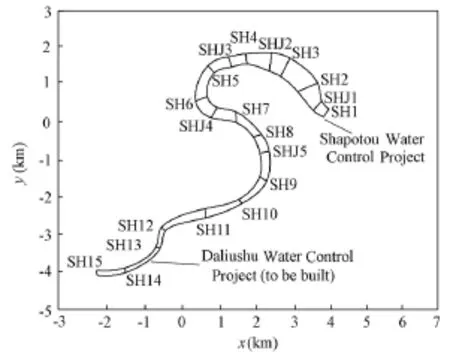
Fig. 1 Plane view of Daliushu-Shapotou Reach in Yellow River

In order to compare the measured data and numerical results, twenty cross-sections were assigned, with a flow direction from SH15 to SH1. The five bends were bend A (from SH15 to SH13), bend B (from SH13 to SH11), bend C (from SH11 to SH7), bend D (from SH7 to SH2), and bend E (from SH2 to SH1). Bends A and B were near the exit of the Heishan Gorge, where the river is deep and narrow with a high flow velocity. The average width in this reach is about 135 m, with the normal water level slope being about 0.03%. Bends C, D, and E were near the Shapotou Dam, where the river is wide and shallow with a slow flow velocity. The average width of this reach is about 300 m, with the normal water level slope being about 0.006%.

Because the cross-section SH1 was located at the convergent part of the study reach, where hydraulic elements vary sharply, it could not serve as the outlet of the simulated area. Otherwise, if the full development boundary condition was used at the outlet boundary, the simulated results would not be stable. In order to use the full development boundary condition, the study reach was extended 40 m from SH1 along the external normal direction.

In the computational domain, along the longitudinal direction (ξ direction), 160 grid cells were set, and along the transverse direction (η direction), 30 grid cells were set. The total number of nodes and cells were 4 991 and 4 800, respectively. The Poisson equation method (Versteeg and Malalasekera 1995) was used to conduct body-fitted coordinate transformation and grid generation. Fig. 2 shows the meshes of the computational domain from SH9 to the outlet.

Fig. 2 Meshes of computational domain from SH9 to outlet

The software Matlab 7.1 was used to program, and the numerical simulations were performed on an IBM work station with an Intel ® Xeon 2.0 GHz core of 4.0 GB of memory. The work station’s operation system was Ghost-Server 2003 SP2. Typical numerical simulation for a typical case took about 42 minutes.

4.2 Verification of flow model and numerical methods

The simulated results show similarities for four cases. Only case 2 was chosen to compare the simulation with measurements.

Three typical cross-sections (SH7, SH5, and SHJ2) were selected to compare the simulated and measured depth-averaged velocities, as shown in Fig. 3. SH7, SH5, and SHJ2 were located in bend D in the study reach, where the left bank is the concave bank, and the right bank is the convex bank. SH7 was at the inlet of the bend, where the maximum velocity is near the concave bank; SH5 was located at the apex of the bend, where the maximum velocity is near the concave bank; and SHJ2 was at the outlet of the bend, where the velocity is close to uniform. Both the measured and simulated velocities are in accordance with the basic rule of the bend flow. Fig. 3 shows the comparison of the depth-averaged velocities calculated using two methods. The first method (Simulation 1) was to use the 2D depth-averaged RNG k-ε model without addition of the circulation flow term, while the second method (Simulation 2) was to use the same model, improved by adding the circulation flow term (improved 2D depth-averaged RNG k-ε model). It was seen that the simulated velocity using the second method is better compared with the measured data than that using the first method, indicating that the improved 2D depth-averaged RNG k-ε model is capable of simulating the effect of circulation flow in natural rivers.

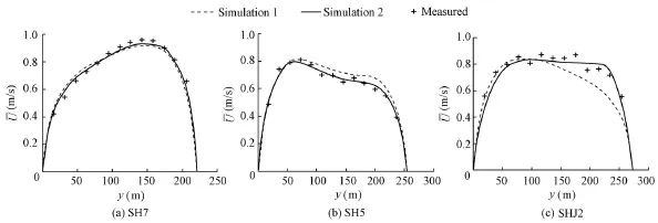
Fig. 3 Comparison of simulated velocities using two methods and measurements

Fig. 4 shows the simulated 2D flow field of the computation domain from SH12 to the outlet. It can be seen that the simulated velocity field abides by the basic rule of water flow in bends, namely, that the maximum velocity appears near the convex bank at the inlet of a bend. It then gradually shifts from the convex bank to the concave bank as water flows downstream. When water flow arrives at the apex of the bend, the maximum velocity takes place near the concave bank of the bend. It then turns from the concave bank to the convex bank gradually again as water flows downstream.

Fig. 5 shows the comparison between the positions of the talweg (where the water depth is the largest along the river width) and the main streamline (where the depth-averaged velocity is the highest along the river width). They coincide for most of the river reach investigated. Generally speaking, the velocity is larger wherever the water depth is larger along the transverse direction. However, the talweg and the main streamline do appear at different locations in the computational domain, such as the reaches from SHJ4 to SH6, from SH4 to SHJ2, and from SH2 to SHJ1 (see Fig. 1). The reach from SHJ4 to SH6 is at thejunction of bends C and D, and there is no obvious straight transition section between the two bends. From SH4 to SHJ2, the river width suddenly increases, while from SH2 to SHJ1 the river width suddenly decreases. From this analysis it can be concluded that when the topography is complex, the maximum water depth and the maximum velocity usually appear at different locations.

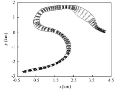
Fig. 4 Simulated 2D flow field of computation domain from SH12 to outle

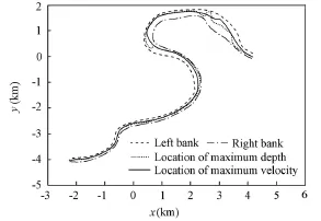
Fig. 5 Comparison of talweg and main streamline positions

The adaptive algorithm was used to automatically determine Manning’s roughness coefficient. To this end, the study river reach was divided into several sub-reaches according to the water surface slope. In this study, numerical tests were conducted to calculate Manning’s roughness coefficient automatically in case 2 (see Table 2). Table 3 shows the longitudinal water surface slope and Manning’s roughness coefficients for three methods of dividing the river reach. In method 1, the study river reach was not divided and Manning’s roughness coefficient of the whole reach was 0.034. In method 2, the study river reach was divided into two sub-reaches based on the water surface slope and Manning’s roughness coefficients of the two sub-reaches were 0.036 and 0.034, respectively. In method 3, the study river reach was divided into four sub-reaches and Manning’s roughness coefficients of the four sub-reaches were 0.036, 0.035, 0.021, and 0.019, respectively.

Table 3 Manning’s roughness coefficients and longitudinal water surface slopes using different methods

Fig. 6 shows the comparison of the water levels simulated using the three methods described above and the field-measured data. The water level simulated using method 3 agrees with the field measurements, while there exists a larger deviation between the simulationsusing methods 1 and 2 and field measurements, with method 1 giving the worst results. Therefore, it can be concluded that the adaptive algorithm for Manning’s roughness coefficient combined with the domain split method can not only save calculation time, but also improve the accuracy of the simulation.

Fig. 7 shows the simulated water levels along the longitudinal direction in the four cases investigated here. The decrease of the water level along the longitudinal direction in all cases investigated is not uniform. A sharp drop of the water level (or water level gradient greater than 0) was found to take place at the upper reach (e.g., from the inlet to SH11, or the first 4 km from the inlet) in all cases. Such a water level drop becomes gradual downstream of SH11 in all cases. It is also seen that the greater the velocity is at the inlet (as in case 4 in Table 2), the greater the total water level drop is.

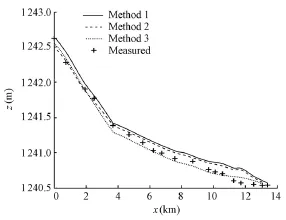
Fig. 6 Comparison of water levels measured and calculated using three methods

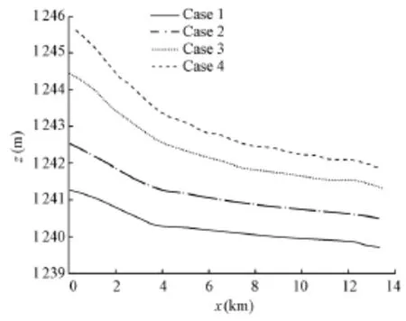
Fig. 7 Comparison of water levels alonglongitudinal direction in four cases

Calculated water surface slopes along the longitudinal direction (main flow direction) increase with the average velocity at the inlet, as shown in tables 2 and 4. Table 4 shows that the longitudinal water surface slope in case 4 is almost 3.6 times that in case 1, while the average velocity at the inlet in case 4 is almost twice that in case 1.

Table 4 Comparison of water surface slopes of four cases

Table 4 also shows the calculated transverse slopes of the water surface at three typical cross-sections (i.e., SH7, SH5, and SHJ2), where the positive value means that the water level at the right bank is higher than that at the left bank, while the negative value means the opposite. The three cross-sections are located near the inlet, apex, and outlet of bend D,respectively, where the left bank is the concave bank, and the right bank is the convex bank. As shown in Table 4, the water level at the concave bank is higher than that at the convex bank at SH5 and SHJ2, while the opposite is true at SH7. In addition, the water surface slope at SH5 is the largest among the three cross-sections. It is concluded that the water level at the concave bank is higher than that at the convex bank downstream of the apex of a bend, while it is quite the opposite near the inlet of the bend. The transverse water surface slope near the apex of a bend is usually larger than that at other positions of the same bend.

In Table 4, it can also be seen that the transverse water surface slope increases very quickly with the average velocity at the inlet. From case 1 to case 4, when the average velocity increases almost twice over, the transverse slope increases by about six times at SH7, five times at SH5, and four times at SHJ2.

5 Conclusions

(1) An improved 2D depth-averaged RNG k-ε model in body-fitted coordinates has been developed in this study. An extra source term considering the circulation flow of a bend has been added in the momentum equations of the model. The numerical examples indicate that the model is capable of simulating natural river flow with continuous bends.

(2) An adaptive algorithm regarding Manning’s roughness coefficient has been proposed. In the algorithm, the study river reach is divided into several sub-reaches based on measured data. Manning’s roughness coefficient in each sub-reach can be calculated automatically. With this algorithm, the computation time is less and the accuracy of the numerical simulation is simultaneously improved.

(3) Water surface slopes were calculated and compared with the field measurements in four cases. It was found that the average velocity at the inlet has significant impacts on both the longitudinal and transverse slopes of the water surface. They both increase with the average velocity at the inlet.

(4) Furthermore, comparison was made between the positions of the talweg and the main streamline. They match for most of the study reach. However, at some positions, such as the junction of two bends and locations where the river width suddenly decreases or increases, they appear at different locations.

Amano, R. S. 1984. Development of a turbulence near-wall model and its application to separated and reattached flows. Numerical Heat Transfer, 7(1) 59-75. [doi:10.1080/01495728408961811]

Guo, Y. K., Wang, P. Y., and Zhou, H. J. 2007. Modeling study of the flow past irregularities in a pressure conduit. Journal of Hydraulic Engineering, 133(6), 698-702. [doi:10.1061/(ASCE)0733-9429 (2007) 133:6(698)]

Guo, Y. K., Zhang, L. X., Shen, Y. M., and Zhang, J. S. 2008. Modeling study of free overfall in a rectangular channel with strip roughness. Journal of Hydraulic Engineering, 134(5), 664-668. [doi: 10.1061/(ASCE) 0733-9429(2008)134:5(664)]

Guo, Y. K., Wu, X. G., Pan, C. H., and Zhang, J. S. 2012. Numerical simulation of the tidal flow andsuspended sediment transport in the Qiantang Estuary. Journal of Waterway, Port, Coastal. and Ocean Engineering, 138(3), 192-202. [doi:10.1061/(ASCE)WW.1943-5460.0000118]

Hayase, T., Humphrey, J. A. C., and Greif, G. 1992. A consistently formulated QUICK scheme for fast and stable convergence using finite-volume iterative calculation procedures. Journal of Computational Physics, 98(1), 108-118. [doi:10.1016/0021-9991(92)90177-Z]

Humphery, J. A. C., and Pourahmadi, F. 1983. Prediction of curved channel flow with an extended k-ε model of turbulence. AIAA Journal, 21(10), 1365-1373. [doi:10.2514/3.8255]

Jing, H. F., Guo, Y. K., Li, C. G., and Zhang, J. S. 2009. Three-dimensional numerical simulation of compound meandering open channel flow by the Reynolds stress model. International Journal for Numerical Methods in Fluids, 59(8), 927-943. [doi:10.1002/fld.1855]

Jing, H. F., Li, C. G., Guo, Y. K., and Xu, W. L. 2011. Numerical simulation of turbulent flows in trapezoidal meandering compound open channels. International Journal for Numerical Methods in Fluids, 65(9), 1071-1083. [doi:10.1002/fld.2229]

Kang, H., and Choi, S. U. 2006. Reynolds stress modelling of rectangular open-channel flow. International Journal for Numerical Methods in Fluids, 51(11), 1319-1334. [doi:10.1002/fld.1157]

Khosla, P. K., and Rubin, S. G. 1974. A diagonally dominant second order accurate implicit scheme. Computers and Fluids, 2(2), 207-209. [doi:10.1016/0045-7930(74)90014-0]

Kimura, I., Onda, S., Hosoda, T., and Shimizu, Y. 2010. Computations of suspended sediment transport in a shallow side-cavity using depth-averaged 2D models with effects of secondary currents. Journal of Hydro-environment Research, 4(2), 153-161. [doi:10.1016/j.jher.2010.04.008]

Launder, B. E., and Spalding, D. B. 1974. The numerical compuation of turbulent flows. Computer Methods in Applied Mechanics and Engineering, 3(2), 269-289. [doi:10.1016/0045-7825(74)90029-2]

Lien, H. C., Hsieh, T. Y., Yang, J. C., and Yeh, K. C. 1999. Bend-flow simulation using 2D depth-averaged model. Journal of Hydraulic Engineering, 125(10), 1097-1108. [doi:10.1061/(ASCE)0733-9429 (1999)125:10(1097)]

Liu, Y. L., and Liu, Z. 2007. Numerical simulation to flows in curved channels. Chinese Journal of Applied Mechanics, 24(2), 310-312. (in Chinese). [doi:1000-4939(2007)02-0310-03]

Molls, T., and Chaudhry, M. H. 1995. Depth-averaged open-channel flow model. Journal of Hydraulic Engrgineering, 121(6), 453-465. [doi:10.1061/(ASCE)0733-9429(1995)121:6(453)]

Nagata, T., Hosoda, T., Muramoto, Y., and Rahman, M. M. 1997. Development of the numerical model to forecast the channel processes with bank erosion. Proceedings of the 4th Japan-Chinese (Taipei) Joint Seminar on Natural Hazard Mitigation, 167-176.

Pezzinga, G. 1994. Velocity distribution in compound channel flows by numerical modeling. Journal of Hydraulic Engineering, 120(10), 1176-1198. [doi:10.1061/(ASCE)0733-9429(1994)120:10(1176)]

Speziale, C. G., and Thangam, S. 1992. Analysis of an RNG based turbulence model for separated flows. International Journal of Engineering Science, 30(10), 1379-1388. [doi:10.1016/0020-7225(92)90148-A]

Sugiyama, H., Hitomi, D., and Saito, T. 2006. Numerical analysis of turbulent structure in compound meandering open channel by algebraic Reynolds stress model. International Journal for Numerical Methods in Fluids, 51(7), 791-818. [doi:10.1002/fld.1159]

Thomas, P. D., and Middlecoff, J. F. 1980. Direct control of the grid point distribution in meshes generated by elliptic equations. AIAA Journal, 18(6), 652-656. [doi:10.2514/3.50801]

Versteeg, H. K., and Malalasekera, W. 1995. An Introduction to Computational Fluid Dynamics—The Finite Volume Method. 1st ed. Harlow: Addison Wesley Longman Limited.

Wu, X. G., Shen, Y. M., Zheng, Y. H., and Wang, P. Y. 2003. 2-D flow SIMPLEC algorithm in non-orthogonal curvilinear coordinates. Journal of Hydraulic Engineering, 48(2), 25-30. (in Chinese).

Yakhot, V., and Orzag, S. A. 1986. Renomalization group analysis of turbulence. I: basic theory. Journal of Scientific Computing, 1(1), 3-51. [doi:10.1007/BF01061452]

(Edited by Yan LEI)

This work was supported by the National Natural Science Foundation of China (Grants No. 11361002 and 91230111), the Natural Science Foundation of Ningxia, China (Grant No. NZ13086), the Project of Beifang University of Nationalities, China (Grant No. 2012XZK05), the Foreign Expert Project of Beifang University of Nationalities, China, and the Visiting Scholar Foundation of State Key Laboratory of Water Resources and Hydropower Engineering Science, Wuhan University, China (Grant No. 2013A011).

*Corresponding author (e-mail: cglizd@hotmail.com)

Received Oct. 17, 2012; accepted May 20, 2013