On Fair Distribution of Discrete Resources
2013-12-19 01:41SunJianxin
绍兴文理学院学报(自然科学版) 2013年3期
Sun Jianxin
(Department of Mathematics, Shaoxing University, Shaoxing, Zhejiang 312000)
1 The Principles and Axioms of Fair Distributing Discrete Resources
A method of fair distributing discrete resources must meet the principles as follows:
A.Equal-for-Members Principle:Each member is equally important for distributing resources,there is no special member who enjoys special preferential rights.
B.Symmetry-of-Department Principle:The resources distributed to each department rely only on the population of the department,and have nothing to do with the serial number of the department(such as subscript).
According to above principles,several axioms can be proposed.As a famous try,M.L.Balinski and H.P.Young put forward the five axioms about seats-distributing[1].After appropriate modification and supplement[2],they are adjusted as the nine axioms about fair distributing discrete resources as following:
Axm.1 Population-monotonicity Axiom:The increasing population of any department would not cause reducing resources of the department.
Axm.2 Resource-monotonicity Axiom:The increasing total number of resources would not cause reducing resources of any department.

Proximity is also known as neutrality.

Axm.5 Scheme-optimality Axiom:The distance in vector space between actual scheme and ideal scheme(i.e.quota) reaches minimum.
Axm.6 Index-universality Axiom:A simple and uniform index of distributing resources is applicable to all possible situation such as any number of departments (m≥2),any population of the department (pj≥1) as well as any number of resources (nj≥0).
Index-universality axiom is equivalent to two axioms:method-transparency axiom and method-universality axiom.Because the most transparent is index-method,therefore method-universality can be replace by index-universality.
Axm.7 Department-unbiasedness Axiom:All deviations between relative unfair-degree and standard value(i.e.1)of each department are equally important(i.e.with equal weighted).
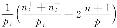
Axm.8 Index-unbiasedness Axiom:If choose index ‘a’ as unfair-degree,must consider both pre-index a-(index before the adjustment) and post-index a+(index after the adjustment),and both are equally important(The most important character of discrete function with arbitrary step).
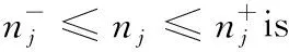
Axm.9 Population-sequentialityAxiom:The sequence of distributing resources is relied on population of corresponding department,i.e.resources allocated to the department with more population can’t less than the department with less population.
Unfortunately the nine axioms mentioned are compatible not all,although they are complete.
2 The Mathematical Model of Fair Distributing Discrete Resources
The meaning of variables in this paper are as follows:
mis total number of departments in the group;
pjis population of j-th department;
pis total population of the group;
nis total number of discrete resources for distributing(nis integer) ;
njis number of discrete resources distributing to j-th department(njis integer) ;


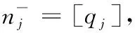
[x]=max{n|n≤x,n∈Z} is lower integer of real numberx;
qj=npj/pis ideal distributing (quota) of j-th department;
bj=qj-njis deviation of actual distributing resources from ideal quota of j-th department;
bj*=qj-[qj]=(qj) is decimal part of quota;
gj=njris covered people by resources of j-th department;
aj=pj-gj=bjris deviation of covered people from population of j-th department;
r=p/nis average representative-rate of group;
rj=pj/njis representative-rate of j-th department;
rj-=pj/nj-is pre-representative-rate of j-th department;
rj+=pj/nj+is post-representative-rate of j-th department;
d=1/r=n/pis average distributing-rate of group;
dj=1/rj=nj/pjis distributing -rate of j-th department;

tj=dj/dis relative distributing-rate of D-to-G of j-th department;
tij=di/djis relative distributing-rate of i-th department to j-th department;

uj=rj/ris relative representative-rate of D-to-G of j-th department;
uij=ri/rjis relative representative-rate of i-th department to j-th department;


The main equality describing relation between variables:
gj=njr,nj=gjd,rd=1;
pj=njrj,nj=pjdj,rjdj=1;
dj=tjd,rj=ujr,tjuj=1;
pj=qjr,qj=pjd;
pj=njrj=qjr=gjuj;
nj=pjdj=gjd=qjtj.
For the problem of fair distributing discrete resources a discrete optimized model can be constructed.As an index vectorX=(x1,…,xm)choose resource vectorN=(n1,…,nm),population vectorP=(n1r,…,nmr),distributing-rate vectorD=(d1,…,dm),representative-rate vectorR=(r1,…,rm),relative distributing-rate vectorT=(t1,…,tm),or relative representative-rate vectorU=(u1,…,um).As an ideal index vectorX0=(x01,…,x0m) choose respectivelyN0=(q1,…,qm),P0=(p1,…,pm),D0=(d,…,d),R0=(r,…,r),T=(1,…,1 ),orU=(1,…,1).The distance of vector space is weighted norm ‖·‖k,w(a,h)=‖·‖k,h(a),here
(2.1)

(2.2)
Lemma 2.1‖P-P0‖k,h(p)=r‖N-N0‖k,h(p)=rc1‖D-D0‖k,k+h=c1‖T-T0‖k,k+h,
c1={p(k+h)/p(h)}1 / k.

Similarly,we can prove the lemma 2.2 and their deductions as following: (proof is omited)
Lemma 2.2All distances are equivalent ifnj>0(j=1,2,…,m)
‖N-N0‖k,h(N)=d‖N-N0‖k,h(N)=dc2‖R-R0‖k,k+h(N)=c2‖U-U0‖k,k+h(N),
c2={n(k+h)/n(h)}1/ k.
Deduction 2.3‖P-P0‖k,0=r‖N-N0‖k,0=rc1‖D-D0‖k,k(P)=c1‖T-T0‖k,k(P),
c1={p(k)/m}1 / k.
Deduction 2.4‖N-N0‖k,0=d‖P-P0‖k,0=dc2‖R-R0‖k,k(N)=c2‖U-U0‖k,k(N),
c2={n(k)/m}1/ k,nj>0.
According to lemma 2.1 and 2.2,it is easy to get some formulas of equivalent distances:
(1)‖P-P0‖k,h(P)=r‖N-N0‖k,h(P);
(2)‖N-N0‖k,h(P)=c1‖D-D0‖k,k+h(P),c1={p(k+h)/p(h)}1 / k;
(3)‖N-N0‖k,h(N)=d‖P-P0‖k,h(N);
(4)‖P-P0‖k,h(N)=c2‖R-R0‖k,k+h(N),c2={n(k+h)/n(h)}1/ k;
(5)‖T-T0‖k,h(P)=r‖D-D0‖k,h(P);
(6)‖U-U0‖k,h(N)=d‖R-R0‖k,h(N).
Besides the 6 kinds of equivalent distance in lemma 2.1,and 2.2,there exist just 4 kinds of equivalence distance with parameterk=∞:
(7)‖N-N0‖∞,h(N)= ‖N-N0‖∞,h(P)= ‖N-N0‖∞,h(D)= ‖N-N0‖∞,h(R),h∈{0,1,2};
(8)‖P-P0‖∞,h(N)= ‖P-P0‖∞,h(P)= ‖P-P0‖∞,h(D)= ‖P-P0‖∞,h(R),h∈{0,1,2};
(9)‖D-D0‖∞,h(N)= ‖D-D0‖∞,h(P)= ‖D-D0‖∞,h(D)= ‖D-D0‖∞,h(R),h∈{0,1,2};
(10)‖R-R0‖∞,h(N)= ‖R-R0‖∞,h(P)= ‖R-R0‖∞,h(D)= ‖R-R0‖∞,h(R),h∈{0,1,2}.
3 The Relation between Models and Indexes
Firstly,classic distributing method of discrete resources can be divided into two categories: model-method and index-method. Secondly the index-method still can be devided into two kinds: one is all-index method,the other is half-index method. So called all-index method means that the distributing each resource is according to the index such as d’Hondt Method. So called half-index method means that after pre-distributing the distributing each remaining resources is according to the index such as Hamiltonian Method.
Furthermore method will be different if index different. So many method is directly named as index. In fact,index is a real monotone discrete function ofnjwith parameterspj,p,n. that is
Ij=f(nj;pj,p,n),j=1,2,…,m.

Many method of resource-distributing can be obtained from some discrete optimalized model of resource-distributing.
Similarly from every model of resource-distributing may be obtained a method which index of max-losser priority or min- gainer priority is corresponding to the model.
Once the parameters of model are determined,the corresponding index are determined as well. In fact,there is the following proposition:
Theorem 3.1Let the optimization model of fair distributing discrete resources
min‖X-X0‖k,h(A),h∈{0,1,2}

Then it’s corresponding index of max-loss priority is
(3.1)
ProofIfk=0,by the property of norm it is available that

(C1)‖X1-X0‖0,h(A)< ‖X2-X0‖0,h(A);
By (C3) we can know that the proposition is true whenk=0.
Ifk=1 or 2,by definition of norm

(C1)‖X1-X0‖k,h(A)< ‖X2-X0‖k,h(A);
By(C3)we can know that the proposition is true whenk=1 or 2.
Ifk=∞,by property of norm we have
(C1)‖X1-X0‖∞,h(A)< ‖X2-X0‖∞,h(A);
There exist four cases as following:


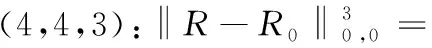
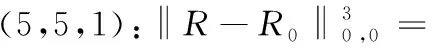
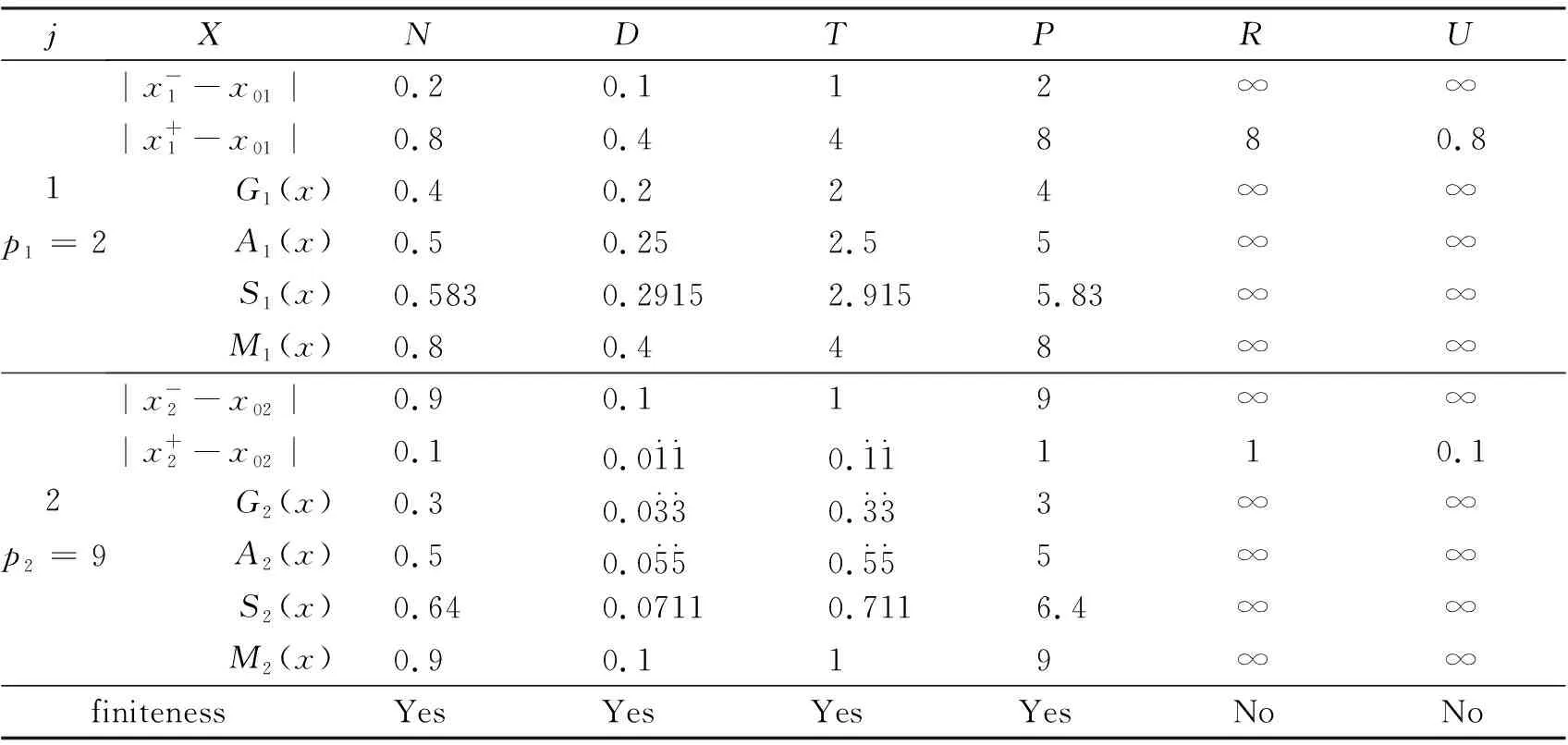
ForX=N,(C5) is equivalent to 1-b1<1-b2,that isb2 Similarly,we can prove the proposition be true forX=P,R,U. The proof is omited. Comprehensive of four cases,whenk=∞,h∈{0,1,2} So far,the Theorem 3.1 is proved. Theorem 3.2Let the optimization model of fair distributing discrete resources min‖X-X0‖k,h(A),h=∞ Then it’s corresponding index of max-loss priority is (3.2) This proposition can easy be obtaind from (3.1) ash→∞. The proof is omited. Put out several deductions and their proofs are omitted: According to lemma 2.1 and 2.2 and their special cases,it is shown there exist 10 kinds of equivalent distance,in which only four kinds such as (1)(3)(5)(6) with different variables and same parameters; There are two kinds such as (2)(4) with different variables and different parameters; There are 4 kinds such as (7)(8)(9)(10) with same variables and different parameters. It is clear that two equivalent indexes occurred if and only if there are two equivalent distances with different variables and the same parameters. It is not difficult to know that D-indexes is equivalent to the T-indexes,R-indexes is equivalent to U-indexes; Although P-indexes equivalent to N-indexes,but considering the symmetry is helpful to compare,so both retained. In order save space,here only to be given a table of relation between index and model with parameterh=0,see Table 3.1. Table 3.1 the relation between parameters of model and index Imax or Imin(h=0) By lemma 2.1 and 2.2,‖N-N0‖0,h (P)= ‖D-D0‖0,h (P),‖P-P0‖0,h (N)= ‖R-R0‖0,h (N),it means that vector spaces described by different distances are overlapping.In order to convenient,below is no longer considered the caseX∈{N,P}&k= 0. The General weighted norms withh>0 except equivalent distance (2)&(4) are biased to departments.Hence they are not fair. So below are confined to consider all cases with parameterh= 0. It is not difficult to prove the following propositions: Theorem 4.1The population-monotonicity (Axm.1) which be equivalent to population- sequentiality(Axm.9) is satisfied if and only if by the solution of following model: ProofA)At first to prove that Axm.9 is satisfied if and only if by the solution of model: (4.1) A1)Consider thatX=D,k=1,let (n1,n2,…,nm)(m≥2) is the solution of the model: (4.2) Suppose thatp1>p2,then mustn1≥n2because there exist only two cases in the process of distributing: There exist no other case. Easy to know thatn1≥n2is holding from beginning to the end. So far we had proved thatn1≥n2ifp1>p2for the model (4.1) asX=D,h=0,k=1. Suppose thatp1>p2,then mustn1≥n2-1 in the middle of process andn1≥n2in the end because there exist only four cases in the process of distributing: There will must ben1≥n2because next remaining resource don’t allocate to department 2. Hence may back to (1) ifi>2,or turn to (4) ifi=1. At this time a remaining resource will allocate to department 2 and the casen2=n1+1 is occurred. Then turn to (3); In fact,from the known conditionS2>S1(refer to (2)) deduced several equivalent inequalities as following: Ifm=2,d=n/(p1+p2), then (C3)is equivalent to (C4)n>4n0+2; (C5)Δ=n-n1--n2-=n-2n0-1>2n0+1≥1. Ifm>2,might as well suppose that the last distributing of department 3~mis (n3,…,nm),letn*=n-n3-…-nm,then(C3) is equivalent to (C7)Δ=n*-2n0-1>2n0+1≥1. Thus next remaining resource don’t allocate to department 2 until department 1 add at least 1,the process may back to (3) ifSi=max{Sj}&i>2 ,else turn to (1) or (2) ifSi=max{Sj}&i=1; It is clear thatn1≥n2still is holding even if a remaining resource is allocated to department 2. Thus the process may back to (4)ifn1>n2or turn to (1) or (2) ifn1=n2. There exist no other case. Easy to know thatn1≥n2is holded in the end. So far it has been provedp1>p2impliesn1≥n2in model (4.1) ask=1 or 2 (X=D,h= 0). B)Secondly to prove that Axm.9 is equivalent to Axm.1. In the fact,the casep1>p2withn1≥n2happens up to now,if some years ago the population of department 1 just equal to population of department 2 today,i.e. p1′=p2,n1′=n2. (*) For department 1 the resources increased fromn2ton1as its population increasing fromp2top1. So Axm.9 is equivalent to Axm.1. But for discrete problem cannot guarantee equality(*) always exists. In general,to prove it must use reduction to absurdity. It can be divided into two propositions: B1)One hand,Axm.1 implies Axm.9. If not so,assuming that does not meet the Axm. 9,which means that at certain time there exist department 1 and 2 such thatp1>p2andn1 B2)The other hand,Axm.9 implies Axm.1.If not so,assuming that does not meet the Axm.1,which means that after a few years,there is a department 1 which resources is decreasing as it’s population increasing,namelyp1′>p1andn1′ C)So far it has been proved the Theorem 4.1 is true ifX=D. Pay attention tor=1/d,Aj(r) =1/Hj(d),refer the table 3.1 and the lemma 2.1& 2.2 it is easy to know that the Theorem 4.1 is true as well ifX∈{R,T,U}. Theorem 4.2The resource-monotonicity(Axm.2)is satisfied if and only if by the solution of following model: min‖X-X0‖1,0,, st.∑nj=n,nj∈Z0+,X∈{D,R,T,U}. ProofIt is clear that premise of resource-monotonicity ism≥3. Firstly we consider thatX=D,k=1(h=0). To prove it only ifm= 3,and the rest by analogy. ‖D3-D0‖1,0≤‖D1-D0‖1,0,‖D3-D0‖1,0≤‖D2-D0‖1,0. (4.3) (4.4) In fact,whether inequality(4.3) or inequality(4.4) are equivalent to following inequality A3(d)≤A1(d),A3(d)≤A2(d). (4.5) So the proposition is correct asX=D. Pay attention tor=1/d,therefore the proposition is correct asX=R. In fact the conditionk=1 is both sufficient and neccesary. It is enough to prove that cannot guarantee that model meet resources monotonicity,ifkis not equal to 1 (k=0,2 or ∞).For example,ifk=2(h=0) the model may not meet resources monotonicity,because the inequilities: ‖D3-D0‖2,0≤‖D1-D0‖2,0, ‖D3-D0‖2,0≤‖D2-D0‖2,0. (4.6) Their equivalent conditions are (4.7) If you want to prove to the model meet resources monotonicity,must deduced the following inequality (4.8) from (4.6): (4.8) Their equivalent conditions are (4.9) But must add conditionpi≥p3(i=1,2) to deduce (4.9) from (4.7). It means that the all population of departments must be equal by sysmetry. In general case the populations are different(at least is not all the same). We can also prove proposition by counter-example.In particular forX=R,k=∞,h=0 provide the counter-example as follows: m=3,p1=p2=23,p3=54,p=100. (This example still is applied in case ask=2,the result is in brakets at the end of every lines.) Whenn=10,try to compare three schemes: (denote max {A,B,C} asA∨B∨C) (1) (2,2,6):‖R-R0‖∞,0= (23/2-10)∨(23/2-10)∨(10-54/6)=1.5∨1.5∨1 =1.5; (5.5) (2) (2,3,5):‖R-R0‖∞,0= (23/2-10)∨(10-23/3)∨(54/5-10)=1.5∨7/3∨0.8=7/3; (8.33) (3) (3,3,4):‖R-R0‖∞,0= (10-23/3)∨(10-23/3)∨(54/4-10)= 7/3∨7/3∨3.5=3.5. (23.14) Obviousely the optimal solution is (2,2,6). Asn=11,try to compare three schemes: (1) (2,2,7):‖R-R0‖∞,0= (2) (2,3,6):‖R-R0‖∞,0= (3) (3,3,5):‖R-R0‖∞,0= It is easy to know that optimal solution of the model becomes to (3,3,5),i.e.the resources of department-3 decreased from 6 to 5 as total resources is increasing from 10 to 11. ForX=R,k=0(h=0) we provide the counter-example as follows: m=3,p1=p2=43,p3=14,p=100. Whenn=10,let’s try to compare three schemes: Obviousely the optimal solution is (4,4,2). Asn=11,let’s try to compare three schemes: It is easy to know that optimal solution of the model becomes to (5,5,1),i.e.the resources of department-3 decreased from 2 to 1 as total resources is increasing from 10 to 11. As a result,the Theorem 4.2 is true. ProofConsider thatX=N,k∈{1,2,∞},h=0.Give an assumption thatN*= (n1,n2,…,nm) (m≥2)is the solution of the model as following: (4.10) If not so,then two cases may occue: (for examplek=1) |(n1-d) -q1| +|(n2+d)-q2|+…=m‖N’-N0‖1,0. Ifc≤d,similarly can prove schemeN″=(n1-c,n2+c,…,nm) is beter thanN*=(n1,n2,…,nm) which is contradicted with assumption. d+(1-b1)+…+bm-d+1+…+bm>(1-b1) +…+(1-bm-d+1)+…+(1-bm)= So far the Theorem 4.3 had been proved ask=1.The propopsition can be proved similarly ask=2 andk=∞, the proof is omited. But the proposition is not true instead ofk=0. In fact,there exist the counter-example as following: counter-example 4.1Letpj=2(j=1,2,…,9),p10=82 andn=10. Find out the solution of the model: (4.11) and verify the solution of model (4.11) don’t meet resource- proximity. Solutionp=∑pj=9(2)+82=100.d=n/p=10/100=0.1.qj=pjd=0.2(j<10) andq10=8.2. It means just the model(4.10) satisfies resource-proximity. As a result,the Theorem 4.3 is true. min‖P-P0‖k,0,, ProofPay attention to the model as follows: (4.12) Theorem 4.5The scheme-optimality(Axm.5)is satisfied if and only if by the solution of following model: ProofConsider that all of ‖X-X0‖k,hare unfair-degrees of resources-distributing if and only ifX∈{N,P,D,R,T,U}. Because norm ‖X-X0‖k,hbecomes general distance of vector-space ifk=2,soXis nearest index-vector from ideal pointX0ifXto be the solution of following model: Therefore the solution X of the model is the optimal. As a result,the Theorem 4.5 is true. Theorem 4.6The index-universality (Axm.6) is satisfied if and only if by the solution of following model: ‖X-X0‖k,h≠∞, X∈{N,P,D,T},k,h∈{0,1,2,∞}. In this case the departments 1 and 2 mentioned above can be compared to determine the distributing-scheme according to their distances. As a result,the Theorem 4.6 is true.Consider following example as real evidence. Example 4.2Letm=3,p1=2,p2=9,p3=89(p=100).n=10,r=10(d=0.1). Calculate all distances in table and fill results in corresponding blank space,see table 4.1.(data of 3-nd Dept. are omited) table 4.1 the distance data of example 4.2 Theorem 4.7The department-unbiasedness(Axm.7) is satisfied if and only if by the solution of following model: ProofIt is clear that the weighted value of every department is same,i.e.wj=1/mifh=0 andX=T.It implies that all deviations of relative distributing-rate of each department from standard-value 1 are equally important. By lemma 2.1 the proposition is still correct whenX=UorDorR. As a result,the Theorem 4.7 is true. In addition,Axm.7 is equivalent to Axm.1 or Axm.9 because their model are the same. Theorem 4.8The index-biasedness (anti-Axm.8) is satisfied if and only if by the solution of following model: ProofConsider that the other possible beyondX∈{N*,P*,D*,R*,T*,U*} and *∈{+,-}.It means that Some departments use pre-distributing index,some departments are post-distributing index. Consider a resource to transfer between two kinds of departments,and will appear at the same time with pre - after index. As a result,the Theorem 4.8 is true. Temporarily take no account of axiom 8,according to the Theorem 4.1~4.7 each of axioms(Axm.1~Axm.7) can to show by the different ranges of variable with parameter of model in Veen Diagram as folowings. So lemma 5.1 is true(refer the diagram 5.1). Lemma 5.1About axioms of resource-distributing there are mainly some conclusions as follows: (1)The Axm.1(population-monotonicity) is equivalent to the Axm.7(department- unbiased- ness). In order to simplify,Axm.7 always is replaceded by Axm.1 later and Axm.7 is omited; (2)The solution of model which meet the Axm.2(resource-monotonicity) satisfies Axm.1(department-unbiasedness); (3)The solution of model which meet the Axm.3(resource- proximity) satisfies the Axm.6(index- universality); (4)Axm.3(resource- proximity) in {N,D,T} is equivalent to Axm.4(population - proximity) in {P,R,U}. (5)Axm.1(population-monotonicity) is incompatible with Axm.3(resource- proximity) or Axm.4(population -proximity).By (2) it implies that Axm.2(resource-monotonicity) is incompatible with Axm.3(resource-monotonicity) or Axm.4(resource-proximity) as well. (6)Axm.2(resource-monotonicity) is incompatible with Axm.5(scheme-optimality). Diagram 5.1 Veen Diagram which subsets are region of parameters satisfied Axm.1-7 Theorem 5.2(Impossibility Theorem) A method of resource-distributing which will be satisfy the Axm.2 (resource-monotonicity) and the Axm.3 (resource-proximity) at the same time is not possible. ProofBy the diagram 5.1 it is easy to know that the intersection of region meat Axm.2 with region meat Axm.3 is empty set. So the theorem 5.2 is true. Deduction 5.3A mothod of resource-distributing which will be satisfy the Axm.1 (population- monotonicity),Axm.2 (resource-monotonicity),Axm.3 (resource - proximity),Axm.4 (population - proximity) and Axm.5 (scheme-optimality) at the same time is not possible. Deduction 5.4A mothod of resource-distributing which will be satisfy the Axm.1 (population- monotonicity),Axm.2 (resource-monotonicity),Axm.3 (resource-proximity),Axm.4 (population-proximity),Axm.5 (scheme-optimality),Axm.6 (index-universality) and Axm.8 (index-unbiasedness) at the same time is not possible. Since there exist no method to satisfy all axioms of resources-distributing,we are able only to pick out the extreme system of compatible axioms ( ESCA for short ) in the seven axioms Axm.1~6 & 8(Axm.7 and Axm.9 are redundant) which mentioned more or less in the resources- distributing problems. Might as well assume that the seven axioms are equally important. It is easy to obtained the ESCA by lemma 5.1 as follows(as far as possible choose the Axm.8): (1)ESCA1={Axm.1,2,6,8}={population-monotonicity axiom,resource-monotonicity axiom,index- universality axiom,index-unbiasedness axiom}; (2)ESCA2={Axm.1,5,6,8}={population-monotonicity axiom,scheme-optimality axiom,index-universality axiom,index-unbiasedness axiom}; (3)ESCA3={Axm.3,5,6,8}={resource-proximity axiom,scheme-optimality axiom,index- universality axiom,index-unbiasedness axiom}; (4)ESCA4={Axm.4,5,6,8}={population-proximity axiom,scheme-optimality axiom,index- universality axiom,index-unbiasedness axiom}. According to the theory about fair distributing discrete resources mentioned above,the author obtains the optimal methods in four types of resources(see[3]).The main results are as following: The optimal method is W- method for distributing seats without fixed size which index isWj=d-Aj(d); and the optimal method is S- method for distributing seats with fixed size which index isSj=Wj/pj. Hamiltonian method is a good method,but applies only to distributing non-permanent discrete resource. About the fair distributing discrete resources,the summarized results are in table 7.1. Tab.7.1 The Optimal Methods of Distributing Different Resaurces Reference: [1]Balinski M L,Young H P.Fair Representation: Meeting the Ideal of One Man,One Vote[M].Newhaven:Yale University Press,1982:191, [2]Sun Jianxin. Compatibility & completeness of Axioms about Seats Distribution[J].Mathematics in Practice and Theory,2011,41(4):78-84. [3]Sun Jianxin. The Optlmal Methods of Distribution of Discrete Resources[J].Journal of Shaoxing University,2013,33(7):12-16.


4 The Relationship between Axioms and Models


5 The Proof of Impossibility Theorem

6 Extreme System of Compatible Axioms
7 The further results