A new methodology for the CFD uncertainty analysis*

YAO Zhen-qiu

School of Naval Architecture and Ocean Engineering, Jiangsu University of Science and Technology, Zhenjiang 212003, China, E-mail: yaozq_just@126.com

SHEN Hong-cui

China Ship Scientific Research Center, Wuxi 214082, China

GAO Hui

School of Naval Architecture and Ocean Engineering, Jiangsu University of Science and Technology, Zhenjiang 212003, China

A new methodology for the CFD uncertainty analysis*

YAO Zhen-qiu

School of Naval Architecture and Ocean Engineering, Jiangsu University of Science and Technology, Zhenjiang 212003, China, E-mail: yaozq_just@126.com

SHEN Hong-cui

China Ship Scientific Research Center, Wuxi 214082, China

GAO Hui

School of Naval Architecture and Ocean Engineering, Jiangsu University of Science and Technology, Zhenjiang 212003, China

(Received August 4, 2011, Revised September 6, 2012)

With respect to the measurement uncertainty, this paper discusses the definition, the sources, the classification and the expressions of the CFD uncertainty. Based on the orthogonal design and the statistics inference theory, a new verification and validation method and the related procedures in the CFD simulation are developed. With the method, two examples of the CFD verification and validation are studied for the drag coefficient and the nominal wake fraction, and the calculation factors and their interactions which would significantly affect the simulation results are obtained. Moreover, the sizes of all uncertainty components resulting from the controlled and un-controlled calculation factors are determined, and the optimal combination of the calculation factors is obtained by an effect estimation in the orthogonal experiment design. It is shown that the new method can be used for the verification in the CFD uncertainty analysis, and can reasonably and definitely judge the credibility of the simulative result. As for CFD simulation of the drag coefficient and the nominal wake fraction, the results predicted can be validated. Although there is still some difference between the simulation results and the experiment results, its approximate level and credibility can be accepted.

CFD, uncertainty, verification, validation

Introduction

For a long time, research of ship performance relies on the technology of tank test. With the development of computer and hydrodynamics, numerical simulation gradually has become the important tool in ship hydrodynamics research, and the preliminary objective condition to set up the numerical towing tank has been achieved. Uncertainty analysis is a method of evaluation on confidence level of measurement or numerical simulation, which is based on the theory of probability and mathematical statistics, and also the important basic research work of test and numerical calculation. It is one of the numerical towing tank technique core tasks to establish the method of reliable evaluation on the confidence level of prediction results of ship CFD. Tank test uncertainty analysis and assessment technology has been gradually improved and has been formed the basic complete uncertainty recommend rules[1]. Unfortunately slow progress in the uncertainty study of numerical simulation has been made for different understanding in of existing concept, theory and methods.

In 1986, Roache et al.[2]suggested for the first time that it is essential to assess the calculation accuracy of a numerical simulation, thus started the uncertainty study of the numerical simulation method of verification and validation. In 1998 Roache published his monograph on the CFD verification and validation, which systematically discusses the CFD uncertainty analysis evaluation process. AIAA also promulgated the CFD uncertainty analysis evaluation procedures in the same year[3]. On the basis of Coleman and Stern’s[4]pioneering work, ITTC promulgated the recommended rules[5]in 1999 and the amendment proposed rules[6]in 2002. Simonsen and Stern[7]studied the digital simulation uncertainty of the Osaka ESSOflow field using the rules recommended by ITTC. Van et al.[8]analyzed the uncertainty of the SUBOFF model flow calculation. Compana et al.[9]validated the CFD uncertainty of a surface combatant bow. Zhu et al.[10], Zhang et al.[11]and Yao et al.[12]analyzed and assessed the uncertainty of the numerical simulation of the SUBOFF model pressure field, and the resistance and the flow fields.

At present, the assessment methods of the prediction result credibility for the ship CFD are mainly confined to the application and the local improvement of the procedures recommended by ITTC, but such basic issues as the uncertainty concept, the basic theory and the analysis evaluation methods were not systematically studied.

In the interim procedures recommended by ITTC, the conception that the numerical simulation results are random variables is adopted, but not the statistical analysis method, which is the most powerful tools to analyze random variables. The verification process is only on the realized system error correction of the numerical calculation truncation error and the iteration error, and the estimation of uncertainty caused by the correction method. Because other errors or sources of uncertainty were not taken as factors and included, the contribution to the uncertainty of those factors could not be assessed, and one could not judge whether some important factors were missing or whether some unnecessary contributions are included in the uncertainty of the simulation.

The concept of the validation process recommended by ITTC is vague. The turbulence model of the CFD simulation should be an important source of uncertainty, which is the greatest contribution to the CFD uncertainty. However, the turbulence model’s uncertainty evaluation method is not included in the recommended procedure. The interactions between the calculated factors are not considered in the validation method in the recommended procedures, and it is assumed that the calculated parameters are independent of each other. But the interactions will affect the estimation of the combined standard uncertainty and the validation process[13].

The validation judgment process consists of a simple comparison between the CFD simulation results and experiment results, to obtain the relative deviation in percent, thus a vague conclusion of consistency or similarity[11,12]. This is also the common method of validity judgment in the CFD simulation at present.

Based on the orthogonal design and the statistic inference theory, with respect to the measurement uncertainty analysis system, a new verification and validation method and the related procedures in the ship CFD simulation are developed in this paper. Examples of the CFD verification and validation show that this method features the clear physical conception, the sound theoretical basis, the rational analysis method, the complete contents being assessed, the credible result, and the easy operation.

Table 1 The analogy on the uncertainty sources between the experiment and the numerical simulations

1. Definitions and sources of CFD uncertainty

1.1 Definitions of CFD uncertainty

Because the simulated physical phenomenon isusually not thoroughly understood, and in the process of the simulation there may be many unforeseen or out-of-control or not correctional influences, the CFD simulation results like the experimental results have the approximation and the dispersion natures, with characteristics of random variables. The randomness of the numerical simulation results is mainly reflected in the fact that the results are different for the same physical parameters.

Similar to the definition of the measurement uncertainty, the CFD uncertaintyU can be defined as: “the parameters associated with the numerical simulation results that indicate the dispersion characterization for reasonable given simulated values.” Or,U is the possible error matrices from the analogue estimate of simulation results, and it represents the estimated range of the simulated true value.

1.2 Analysis of CFD uncertainty source

The key of a correct evaluation of the reliability of the numerical simulation results is an accurate analysis of the uncertainty sources or the error sources. In the numerical method analysis, there are five kinds of uncertainty sources, they are the mathematical model error, the truncation error, the iteration error, the measurement error and the rounding error. The uncertainty sources in the numerical simulation can be analyzed according to the relatively mature methods for the measurement uncertainty sources. (See Table 1)

As shown in Table 1, the two kinds of sources of uncertainty are different. However, there is a common analogy of relationship. Therefore, the sources of uncertainty in the table are likely to contain the vast majority of sources of errors affecting the CFD simulations.

2. Orthogonal design method and variance analysis of CFD simulation experiment

2.1 Fundamental concept in orthogonal design of CFD simulation experiment

(1) Calculation factor

The calculation factor refers to the uncertainty source of the simulation process from the mathematical model (such as the governing equations, the initial conditions, the boundary conditions, the turbulence model, etc.) and the numerical methods (such as the meshing, the discrete format, the solution method for the discrete equations, etc.).

(2) Level

The level refers to the state of the calculation factor, for instance, the various turbulence models in the RANS equation, the different mesh numbers and the division methods, the discrete models, etc..

(3) Calculation condition

The collocation of a set to investigate the controlled factors fixed on a certain level is defined as the simulation calculation condition. The simulation result refers to the statistical average obtained from the reproducibility calculation when the calculation condition for a certain physical quantity changes. The optimal estimation is refers to the simulation result under the optimal calculation conditions.

(4) Effect and interaction

The effect of a calculation factor refers to the difference in the simulation results caused by the level change of the controlled factors. Beside the influence of single factors, the communal influence of factors on the simulation results is defined as the interaction.

(5) Simulation error

The error refers to the difference between the simulation result and the true value, namely, the overall effect of all calculation factors and their interaction. In order to minimize the error, the most influential factors must be the controlled factors. The simulation error could be attributed to the controlled calculation factors and the out-of-controlled calculation factors, for which, the latter is called the error for short.

2.2 Orthogonal design method of CFD simulation experiment

The orthogonal design method refers to the method used in a physical test involving multiple elements. Provided that the numerical simulation could be regarded as a virtual physical test, then this method may as well be used to design and analyze the virtual test process and the results. The orthogonal design of the CFD simulation experiment refers to the process in which the reproducibility calculation design the socalled repeated sampling sample is done through the orthogonal array scale.

Firstly the calculation factors to be examined should be divided into the controlled calculation factors and the out-of-control calculation factors. The formers are the major elements that affect the simulation result, and the latters include all minor elements other than the controlled calculation factors. Provided that there is something irregular in the statistical checking, further modification is needed. In other words, the simulation test design should be altered, the controlled calculation factors should be altered and so should the calculation and analysis until the controlled factors do significantly affect simulation result.

When the controlled calculation factors are chosen, the level of the factors should be set in a suitable range, and the variable ranges which depend on the demand and possibility of the simulation test and the actual problem.

When the controlled calculation factors and their interaction and the level are set, the orthogonal array should be chosen to ensure that all controlled factors and some blank columns are included. The statement heading should be designed in a way that the contro-lled factors and the interaction scheduled to be examined in every column should not be overlapped in the effect. Accordingly, every row represents a calculation project in which a set of calculation factors on a certain given level collocate, and all the calculation projects here are repeatedly sampled samples belonging to the simulation test under a statistical control.

2.3 Variance analysis method of CFD simulation experiment

The variance analysis refers to a method which distinguishes the experiment results affected by different factor level (including interaction) changes or errors[14]. TheF test is the basis of the variance analysis, and is mainly used to check whether there is a significant difference among levels of calculation factors.

Assume thatF is the ratio of the average sum of squares of deviations caused by the factor level change and the average sum of squares of deviations caused by errors, as

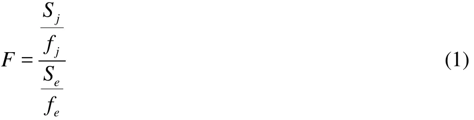
where f is the degrees of freedom andS is the sum of squares of deviations.

Therefore, if the ratio of the effect on the simulation result attribution of the controlled calculation factors and the out-of-control calculation factors can be identified asF , thenF can be used to check whether some major calculation factors are omitted. Meanwhile,Sjand Serepresent the influence of the controlled factors and their interactions on the simulation result and that of the out-of-control factors and their interaction on the simulation result, respectively.

3. Verification process and method in CFD uncertainty analysis

We talk about the “verification” and the “validation” in the uncertainty analysis of the CFD numerical simulation[2,6]. The “verification” is referred to the process of analysis and evaluation sources of the CFD uncertainty and the size of components of the CFD uncertainty, aiming to select the significant influencing calculation factors and the interaction on the simulated result, to find out the optimal combination of the calculation factors, and to acquire a variety of standard uncertainty, combined standard uncertainty and expanded uncertainty for components.

3.1 Verification process in CFD

The verification in the CFD simulation refers to the analysis and evaluation process of all kinds of the CFD uncertainty components. It is used to confirm the significant calculation factors and the interactions, to find out the optimal level collocation or the optimal calculation conditions, and to obtain all kinds of uncertainty components, combined uncertainty and expanded uncertainty.

Fig.1 Flow chart of CFD verification

Verification process of the uncertainty in the CFD simulation based on the orthogonal design could be summarized as in the following flow chart, Fig.1.

3.2 Type A evaluation of standard uncertainty

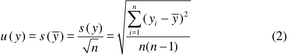
In the process of the numerical simulation under a certain statistical control (such as the orthogonal design), ifis the arithmetic mean value and serves as the estimate value ofy,n is the number of indepe-ndent simulations, i.e., the number of calculations on the orthogonal table,yiis the calculation result of independent simulations ati -th time, the combined standard deviation,Spcan be used as a token and the standard uncertainty of the simulation result is

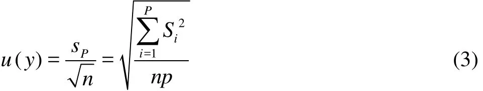
where Sprepresents the combined standard deviation,Sithe sample standard deviation,p the sampling frequency–the number of calculations at the same level, andn the total number of samples.

If the controlled calculation Factor A is put on column j in the orthogonal table, its number of levels beingl , the repeated number of each level being p, and the degree of freedom being fA=l-1, the sum of squares of the deviations sAand uAthe uncertainty of Type A can be calculated and so can sA× Bthe standard deviations and the uncertainty uA× Bof the interaction of the calculation Factors A and B, the out-of-control calculation factor or the random error standard deviations seand uncertainty.

where Sjthe sum of squares of deviations on any column j in the orthogonal table, which can be calculated as follows

In this formula,Ιj,Ⅱj,… represent the sum of y numbers listed on levels “1”, “2”, … and on column j.

As to the interaction, the following formula is used

In this formula,j represents the column of the interaction on the orthogonal table.

3.3 Type B evaluation of standard uncertainty

Wheny is the estimate value of the simulated physical quantityY and is not obtained based on the statistical method, its estimate variance u2(y)and u( y)the uncertainty components for Type B can be evaluated according to the methods such as those based on the historical data, the experience, the adopted error correction formula, the CFD software instruction and other information provided by other documentation.

Based on the information above, the evaluation methods of the uncertainty for Type B are to judge the probable interval (-a, a)of the simulated value, and to presume the probability distribution of the simulated value, by using the confidence level (including the probability) to estimate the coverage factork and then to calculate the uncertainty by the formula as follows

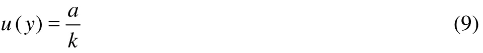
In the CFD simulation, the uncertainty component for Type B comes mostly from the uncertainty caused by known and correctable systerm errors and the imperfection in the correction method. The truncation error and the iterative error of the numerical computation can have an approximate correction and its uncertainty uGand uIcan be calculated by Eq.(9) mentioned above. The mathematical model error and the accumulation of the rounding error that are not clear or uncorrectable will be classified into the uncertainty components of Type A.

The truncation error and the iterative error have a close relationship with the grid model and the discretization form. As to the discrete methods that can meet the stability and convergence conditions, the Richardson extrapolation method adopted by the ITTC recommended procedure can be used to estimate the truncation error and its order. The order of magnitude of the truncation error O( hp)depends on the step sizeh and the orderp . Whenhandp are fixed, its estimate value depends on the approximation method. The difference in the estimate value of the truncation error obtained by different methods should be small, thus it could be assumed that the truncation error obeys the uniform distribution, so its uncertainty is

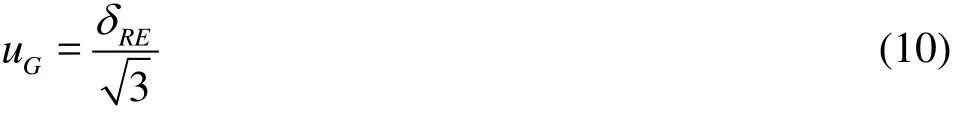
where δREis the interval halfwidth of the probable value of the truncation error.

The iterative error is determined by the iterative methods and the characteristics of the discrete equation’s coefficient matrix. When both of them are fixed, the iterative error is decided by the iterations and the convergence rate of the iteration. Assuming that the probability error distribution caused by a linear change, is in a trianglar distribution, its uncertainty is

where yUand yLare the upper bound and the lower bound of the simulation result that can meet the condition of convergence.

3.4 Calculation of combined standard uncertainty

The uccombined standard uncertainty of CFD is the sum of the variances of all standard component uncertainties ui(x). If there is a significance interaction, the covariance can be used

In this formula,u( xi)and u( xj)are the standard uncertainties of xiand xj,r is the estimated value of the correlation coefficient of xiand xj.

By the methods of the orthogonal design, the u ncertainty like uA× Bof the relative interaction can be calculated, so the covariance can be calculated by directly using uA× Band uB× C.

3.5 Evaluation of expanded uncertainty

For the combined uncertainty (uc)corresponding to the standard deviation, the probability of containing the true value is 68% at the interval of the simulation result y±uc. In some engineering applications, a high confidence probability level is required so that the simulation result falls into the interval, and in the hope that the interval contains with a great probability the simulated value reasonably endowed. To meet this requirement, the expanded uncertainty U can be calculated by multiplying the combined uncertainty and the coverage factork . The following formula is used

Therefore, the result is represented as Y=y±u , where y is the estimate of the simulated value, the interval y-U≤Y≤y+Uis the extent containing with a great probability the reasonably endowedy distribution. The coverage factor k ranges from 2 to 3 based on the confidence level required by the interval y±U. Ifk is 2, it means that the simulation result value which obeys the normal distribution will be in the range of the estimated value ±Uaccording to 95% of probability level. Ifk is 3, the probability level of that interval can reach up to 99%.

4. Validation method and process in CFD uncertainty assessment

After the CFD simulation result is verified, it is usually required to be validated. The “validation” is referred to the process of judging the credibility of the CFD simulation result or a simulation value, and to estimate the possibility of falling into the range of the “error band” of the experiment. The validation may be defined as the comparison process of the statistical characteristic parameters of the simulation results and the experiment results by using the statistical inference theory.

In fact, the results of the physical experiment or the numerical simulation are random variables, and it can be assumed that they obey the normal distribution N(µ,σ). The comparison of two random variables should be made by the concepts and the means of the statistical inference. Strictly speaking, only if the statistical characteristic parametersµand σof the two random variables are equal, no significant differences between them can be validated.

4.1 Statistics inference method for validation

The statistical inference is based on one or several sub-samples to infer or judge the statistical characteristics of its population. The degree of confidence is an important index to measure the reliability.

How to determine the statistical characteristics of the experiment results is not studied in this paper, so here it is assumed that the test result is obtained from the statistical analysis of a large sub-sample and that the population’s expectation and variance are known. Here, the problem is to use the statistical inference method to judge whether the expectation µcand the variance σ2of the numerical simulation population

cinfered from the small sample are the same as the expectation µand the varianceof the population

T of the experiment. If so, then the numerical simulation results are validated.

4.1.1F-test

In the CFD validation process, one first judges whether the variance of the population of the numerical simulationand that of the experimentin the statistical sense is the same or not, by means of the F-test of the statistical inference theory.

The statistical hypothesis goes like this: “There is no significant difference between the two variances of the population generating from the numerical simulation and the physical experiments, that is=”.

Define the followingF variable

T tion, which can be obtained from the database of the benchmark test or the historical information . Suppose that it is known and its degree of freedom is∞.is the estimate of the population σCby a limited number of simulation samples,is the variance estimate of the CFD simulation results,sCis the total sum of the squares of the deviations of the simulation results.f is the degree of freedom,fC=N-1,N is the size of the numerical simulation sub-sample, and is called the program number of the orthogonal design.

The data can be obtained from the verification process of the CFD simulation based on the orthogonal design, as in formulas (16) and (17).

wherel is the level of the calculation factor,p is each level’s repetitive number,y is the simulation results,Ιj,Ⅱj,…are the sum of datay in the column j corresponding to levels “1” “2”,….

For the interaction, we have

Although N cannot be very large, the full factor program information can be obtained because it is a sample from the orthogonal design and the overall information can be obtained from a part of the implementation. So itsF -test confidence is higher than the common sample.

If F＞Fα(fC,∞), then the statistical hypothesis=is untrue, otherwise, it can be believed that=, which means that the population variances of the numerical simulation and the experiment are equal.

4.1.2t -test

From the law of large numbers, the best unbiased estimator of the expectationµ of random variables is the arithmetic mean. So in the validation process, the average of the population of two random variables, i.e., the results of the numerical simulation and the physical experiment, are compared.

From the theory of statistical inference, when the population variances of the two random variables are equal, whether its expected value is equal can be tested by the t distribution. If the two samples are relatively large and equal, even the variances are different, the t -test method can be approximately applied. In fact, the experiment sub-sample is assumed to be a big sub-sample from the benchmark test, and the sub-sample of the numerical simulation is a approximate large sub-sample obtained by the orthogonal design, so the requirements of a relatively large number for the two sub-samples of the same size can be approximately met.

The statistical hypothesis goes like this: “The averages of the population of the sub-samples from the numerical simulation and the experiment are equal,=”. Here,andare the averages of the results from the numerical simulation and the experiment,NCand NTare the sizes of the sub-samples. Define thet variable as

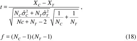
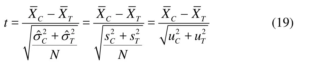
With the general aspects,NC=NT=N, and N is large enough, the formula (18) can be rewritten asin which uCand uTare the combined uncertainty of the CFD simulation and the experiment, respectively.

Considering that the current CFD simulation accuracy can not reach the level of the experiment, so for simplicity, the term uTcan be omitted, formula (19) can be simplified as

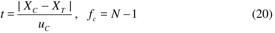
According to thet variable degrees of freedom f and the confidence levelα,ta(fc)the critical value of the variablet can be obtained. If t＜ta, then=, the statistical hypothesis is not untrue. The simulation results can be validated.

If formula (20), in which uTis omitted, replaces formula (19), thet -test conclusion is safer, and i t is not necessary to know the uncertainty or the variance estimate of the experiment. In addition, this direct application without the system error correction for the test method of the simulation results might lead to a dangerous bias. So strictly speaking,and uCin the formula should be the modified results. However, considering the approximate effectes of the two are opposite, the simulation results without modifications and the application of the formula (20) in testing can be acceptable.

Fig.2 Flow chart of CFD simulation result’s validation

4.2 Process of validation

Because the result of the experiment is measured by the etalons calibrated by the measurement standard or the standard in the quantity transfer, there is no need to validate[8]. For the simulation results, it is necessary to judge by the statistical inference method whether the expectation and the variance of the population of the simulation results obtained from a small sub-sample are the same as those of the population of the experiment results. If they are equal, the simulation results are validated.

In this paper, the proposed validation methodology and its process of the CFD numerical simulation can be summarized as in the Fig.2.

4.3 Validation of optimal solution for CFD simulation and estimation of confidence interval

Each controlled calculational factor if it is under the condition of being fixed at some level of matching will form a kind of calculation condition in the simulative process. If under the calculation condition, the minimum numerical simulation deviation is defined as the optimal calculation condition, the optimal matching of the calculative factor can be calculated according to the effect analysis in the orthogonal design, and the simulative result under this condition can be estimated as well, and its interval estimation and credibility should be further carried out.

4.3.1 Determination of optimal calculation condition

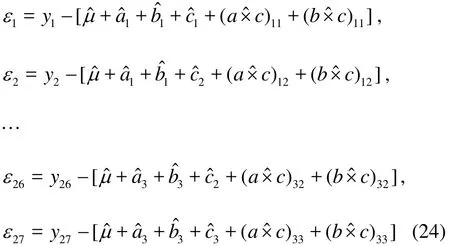
According to the datum structrue formula and the effect estimation of the orthogonal design[14]which aim to reduce the numerical simulation deviation to the least, that is, to make the value ofmˆ , which is the estimate value of the theoretical valuem of the simulative result, as close to the real simulative result y as possible, which means to minimize the residual ε=, therefore we can use ε to substitutey in the orthogonal array for analysis, among which each calculation plan’s( i=1,2,…,N)is the linear sum produced by the arithmetic mean and the effect of each calculative factor and the interaction effect, to determine the optimal calculatine condition according to the smallest εcorresponding to the calculation factor level (interaction included), to determine the estimate value of the simulative result with the application of the effect estimation formula. The detailed calculation methods are as follows:

The assignment mirefers to the total effect towards yiby the level of the controlled factors, i.e., the theoretical value of yj, whose estimation value is

Therefore,µˆis the estimation value of the expectation of the simulation result,is the estimation value of the effect of thei -th calculation factor and the interaction,N is the calculation sample size. Taking the two factors for example,micalculative formula takes the form

4.3.2 Interval estimation of optimal solution and validation method

Under the optimal calculation condition, the numerical simulation result obtained from the orthogonal design plan is the best. The statistical characteristics of the sample population are known, thus making the optimal solution interval estimation itself meaningless. From the validation method, according to the interval estimation of the balance between the numerical simulation result and the experiment result, we can judge whether the optimal solution is confirmed, especially when the results obtained from the simulation process cannot be confirmed.

The question can be rephrased as: the interval estimation of the balance between the numerical simulation result whose population statistical characteristics are known and the mean of the experiment result.p˜ is the possibility that the balance can fall inside the interval at a requested confidence level. According to the normal distribution characteristics, its interval estimation should be

5. Verification and validation examples in CFD simulation

To evaluate the rationality of the verification and validation methods for the ship CFD uncertainty, the same model is used to analyze the submarine resistance and the nominal wake fraction for the ship CFD uncertainty. By comparing these two examples, one may see if the two different simulated physical quantities will influence the verification and validation of the conclusion.

5.1 Computation model

The computation objects are the resistance coefficient CTand the average nominal wake factor ωNof an submarine model with sail and tail appendage[15], adopting the FVM discretization control equation, the momentum equation and the turbulent dissipation rate equation with the second-order upwind scheme discretization, the pressure with the second-order difference scheme, and the pressure velocity coupled iteration with the SIMPLE method. The turbulence models of calculation are the RNG k-ε, the SST k-ωand the RSM, with the computed fields of 4L×1L×πL, the boundary condition: the inlet velocity Vin=V0, at the pressure outlet, the pressure value is equal to the reference pressure Pout=P0, with no slip on the wall, the standard wall unctions, structured grids are adopted, with the grids f closely arranged near the wall, the curvature change spot, the sail and the appendage.

Table 2 Meter design

5.2 Orthogonal design of CFD simulation experiment plan

According to the numerical simulation calculation experience and the error analysis of the submarine resistance and the flow field[13], the main calculation uncertainty comes from the grids and the turbulent mode, but it cannot be determined whether it is acoupling relation between the grids and the turbulence model. Therefore the grid Index A, the thickness of the body-fitted grid innermost layer as the Index B, the turbulent mode Index C, and their interaction factors are chosen as the calculation factors.

Table 3(a) Calculation scheme and results of CTand ωN

The RNG k-ε, the SSTk-ωand the RSM modes are treated as the three levels of turbulence models, which are frequently used in numerical simu6-lations. The three levels of grids are 0.797×10, 1.127×106and 1.594×106. The thickness of the bodyfitted grid on the innermost layer to the wall (corresponding index y+), is set at three levels, respectively, as 0.00002 m (y+=5-40), 0.00004 m (y+=5-60), 0.00006 m (y+=5-90).

The L(313)orthogonal table with interactions

27ischosenforsolvingtheorthogonaldesignproblemwhere there are three factors, and three levels. The design of the meter is indicated as in Table 2.

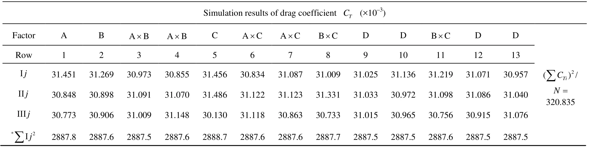
Table 3(b) Calculation scheme and results of CT

Table 3(c) Calculation scheme and results of ωN

Table 4 Variance analysis of drag coefficient CT

5.3 Statistical analysis of computations

The calculation results of the drag coefficient CTand the average nominal wake fraction ωNare listed in Tables 3(a), 3(b), with corresponding results of variance analysis in Table 4 and Table 5.

5.3.1 Statistical analysis of drag coefficient CT

The variance analysis of the drag coefficient CTreveals that the turbulence model, the grid quantity, and the interaction between the grid quality and the turbulence model have a highly significant effect on the calculation results of the drag coefficient. Meanwhile, the grid quality, and the interaction between the grid quantity and the turbulence model have a significant effect on the calculation results.

The factors and interaction of significant effect are kept, such as Factors A, B, C,A×CandB×C , while the others are categorized as error terms. A statistical hypothesis is made that there will be no significant difference in the influence of the controlled factors on the simulation result and of the out-of-control factors, which will be tested byF.

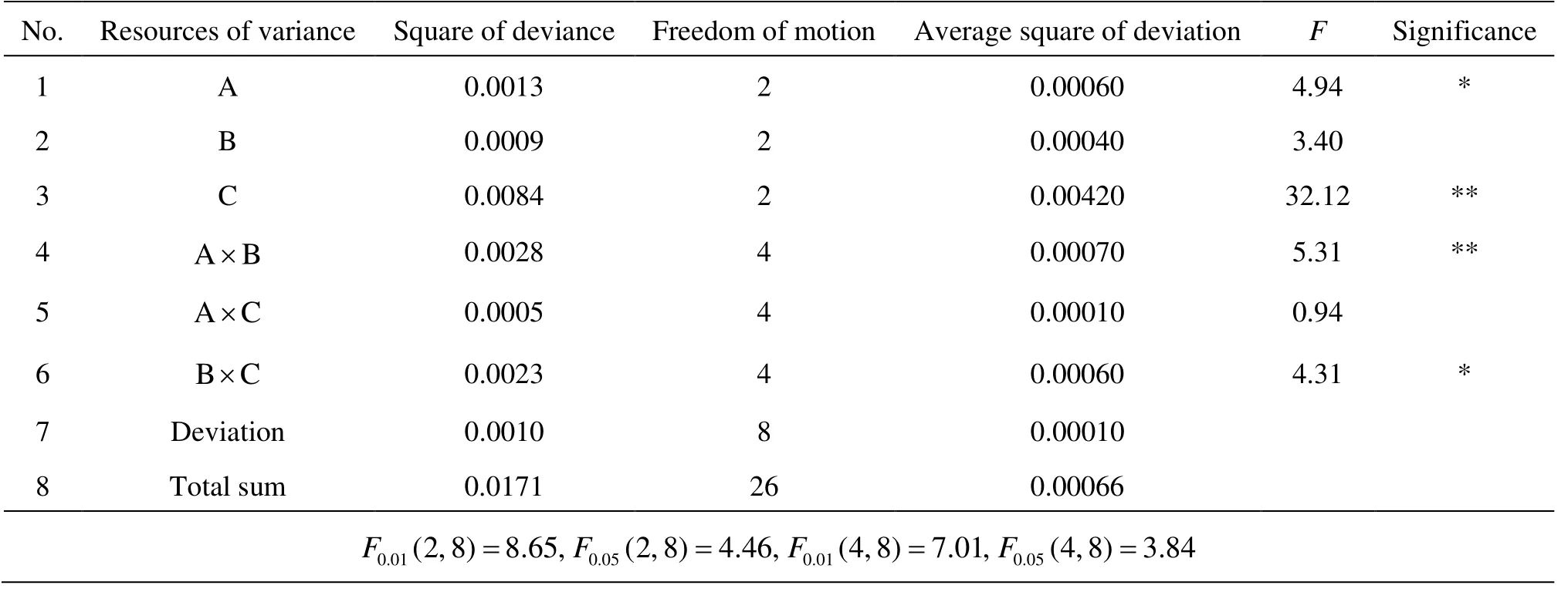
Table 5 Variance analysis of average nominal wake fraction ωN

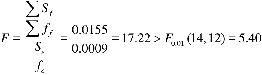
The significant difference proves that the hypothesis is false, which indicates that in the numerical simulation the out-of-control factors, those not categorized as the uncertainty source, can barely contribute to the divergence of the simulation result, which proves the right choice of the controlled factors.

5.3.2 Statistical analysis of average nominal wake fraction ωN

In the numerical simulation of the average nominal wake fraction ωN, the variance analysis reveals that the most influential factor is the turbulence model, followed by the interaction between the grid quantity and the grid quality, and then the grid quantity, the interaction between the turbulence model and the grid quality. All other factors have little influence on the simulation result and can be ignored.

The factors and interaction of significant effect are kept, such as factor A, C andA×B,B×C , while the others are categorized as error terms.

A statistical hypothesis is made: there is no significant difference between the influence of the controlled factors on the simulation results and of out-ofcontrol factors, which will be tested byF

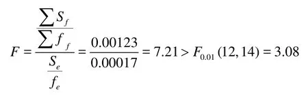
The significant difference shows that the assumption is false.

There is a slight difference in the variance analysis result of the numerical simulation between ωNand CT. The influence of the grid quantity A and the turbulence model C is very significant, while the influence of the thickness of the body-fitted grid innermost layer to the wall B is slight. But the interaction between B and A has a great influence. The interaction between B and C has some influence. This difference proves that for a different physical quantity in the CFD simulation, different controlled calculated factors and interactions should be chosen.

5.4 Drag coefficient CT

5.4.1 Evaluation of CFD uncertainty components of drag coefficient CT

On the basis of the variance analysis result, the CFD uncertainty could be calculated by formulas (2)-(4).

(1) Type A standard uncertainty

Uncertainty of the grid quantity

Uncertainty of the grid quality

Uncertainty of the turbulence model

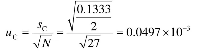
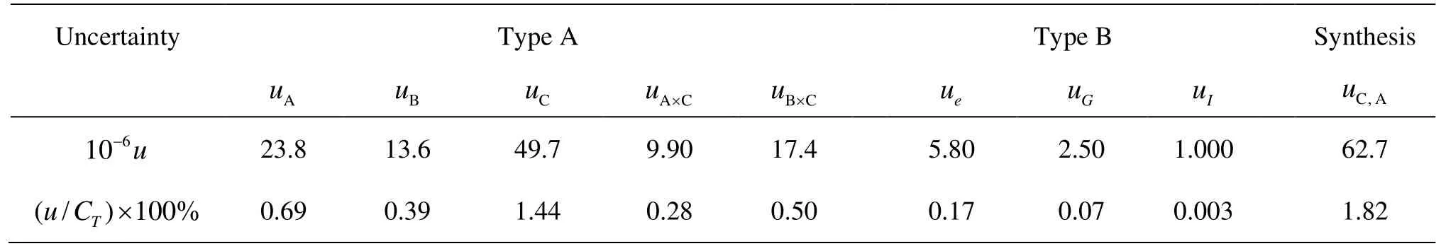
Table 6CTdrag coefficient uncertainty calculative result

Uncertainty of the interaction between the grid quantity and the turbulence model

Uncertainty of the interaction between the grid quality and the turbulence model

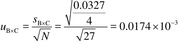
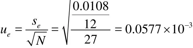
Uncertainty of the out-of-control factors

(2) Type B standard uncertainty

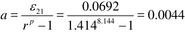
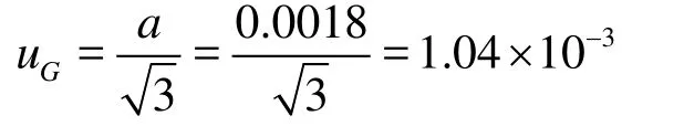
Uncertainty caused by the truncation errors

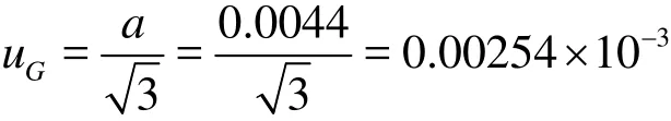
Therein,a is the average truncation error.

Uncertainty caused by the iteration errors

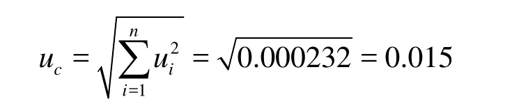
(3) Combined standard uncertainty

(4) Expanded uncertainty

As can be seen in the assessment of the CFD simulation uncertainty of the submarine resistance, in the combined uncertainty uc, the uncertainty component from the turbulence model is the highest, followed by the grid quantity, the interaction between the turbulence model and the grid quality, the grid quality, the interaction between the turbulence model and the grid quantity, the uncertainty component caused by the numerical calculated truncation error and the iteration error. Except for these uncertainty components, the uncertainty components caused by other out-ofcontrol calculated factors are too slight and can be ignored. This conclusion totally agrees with the variance analysis result.

5.4.2 Validation of drag coefficient CT

On the basis of the verification result of the drag coefficient CT(in Table 4 and Table 6), firstly, it is judged whether the population varience between the numerical simulation and the experiment is equal in the statistical sense.

If the variance estimation valueof the experiment is known according to the historical data, and its degrees of freedom will be taken as∞, then formula (15) can be used to judge whether σCand σTare equal. By analyzing the historical data[13], the drag coefficient C’s variance=0.0003960× 10-6

T can be obtained.

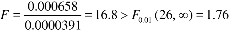
For the statistical hypothesis,=, there are no significant differences between the influence of the factors on the simulation results and the experiment error, according toF to be calculated

But F＞Fα(fs,∞)now, therefore, the statistical hypothesis is untrue, and the two population variances derived from the numerical simulation and the experiment are not equal, which means at present the CFD simulation precision has not reached the level of the experiment. According to this, the conclusion is normal for the current level of the CFD simulation, the experiment cannot be replaced. Therefore, it canbe a hard job to further decrease the difference in accuracy between the numerical simulation and the physical experiment.

Table 7 Effect of the factors at different levels (×10-3)

Table 8 The calculative result of residual with resistance simulation

Secondly, to judge whether the means of thepopulation of the results of the CFD simulation and the experiment are equal in the sense of statistics.

Table 9 Calculative result of uncertainty of average nominal wake fraction ωN

With the experiment’s result[15]of the average known X=3.440× 10-3, for the statistical hypothe-

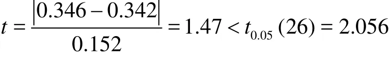
T sis,XC=XT, the t test can be made, that is, by formula (20)

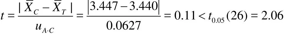
Now t＜ta, which means that the expectation of the numerical simulation and the experiment are equal in the sense of statistics. It shows that even though the two population’s variances (experiment or simulation percision) are different, their mean can be thought to be approximately equal, which means the CFD simulative result can be validated under a lower standard of relax restrictions.

5.4.3 Validation and interval estimation for optimal solution

Take the data of the resistance CFD simulation in Ref.[13] as an example, for the significant calculation Factors A, B and C as well as the significant interactionsB×CandA×C , the estimated results on the effect are shown in Table 7. The theoretical estimated values of each calculation scheme (true value)mnand the residual εm=yn-mnare given in Table 8. According to the design of the table head, we have

From Table 8, the optimal calculation condition is A2, B3, C2 to minimizeε, which means the combination with the grid number of 1.127×106, the grid thickness on the innermost layer to the wall of 0.00006 m, and the SST k-ωturbulent model is the optimal calculative matching mode.

According to formula (21) of the effect estimation, the theoretical estimation value of the optimal simulation result mˆ is

According to formula (23), the possible range of the balance between the numerical simulation value and the experiment result, i.e., the balance interval at the requested confidence level can be estimated. If it is 95%, then tαtakes the value of 2. In the example, the variance of the drag coefficient Cis σˆ2=0.0003960×10–6, the mean is x=3.440× 10-3, there-fore, the estimated result of the confidence interval with the numerical simulation is

The simulation result at the optimal condition is 3.452×10–3. It is thus clear that the difference between the estimated value of the numerical simulation and the result of the experiment would possibly fall inside the interval with 95% probability, so the simulation value can be validated.

5.5 Average nominal wake fraction ωN

5.5.1 Evaluation of CFD uncertainty components of average nominal wake fraction

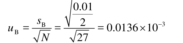
(1) Type A standard uncertainty

Uncertainty of the grid quantity

Uncertainty of the turbulence model

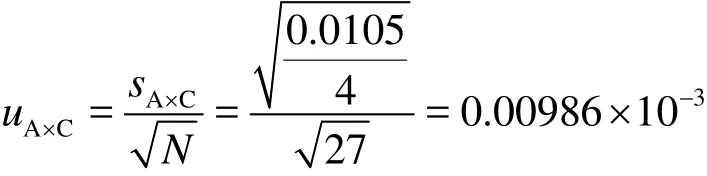
Uncertainty of the interaction between the grid quantity and the grid quality

Uncertainty of the interaction between the grid quality and the turbulence model

Uncertainty of the out-of-control factors

(2) Type B standard uncertainty

Uncertainty caused by the truncation errors

Uncertainty caused by the iteration errors

(3) Combined standard uncertainty

(4) Expanded uncertainty

In view of the CFD simulation uncertainty’s assessment which is about the nominal wake fraction, the result agrees with the variance analysis. In the uncertainty caused by the important calculated factors, the level change is the main one, the uncertainty caused by the out-of-control factors is less influential. However, in the uncertainty caused by the imperfection of the numerical calculation, the error correction method has little effect and can be ignored.

5.5.2 Validation of average nominal wake fraction

The verification of the CFD simulative result of the average nominal wake fraction ωNis shown in Table 5 and Table 9.

It is known from the historical data[13]:= 0.006255, the mean value of the experiment is= 0.342[15]. From formula (15)

It can be seen that the variance is not equal for the numerical simulation and the experiment in the statistical sense like the case for the drag coefficient CT.

Using formula (20) to judge whether the mean of the population from the numerical simulation and the experiment is equal. Thet test is conducted

It is thus clear that in the sense of statistics, the mean of the population from the numerical simulation and the experiment can be seen as equal, therefore, ωNsimulation result is validated.

Comparing the two validation results of CTand ωN, it can be concluded that, though ωNsimulation results are more dispersed and its degree of approximation is not enough, the validation of the numerical simulation can still be achieved with the increase of the experiment’s uncertainty.

6. Conclusions

The statistical concepts of the uncertainty verifycation and validation in the CFD simulation are analyzed in this paper, and the uncertainty sources in the CFD simulation test are analysed. Based on the orthogonal design and the statistical inference analysis, a new verification and validation method and the related procedures in the CFD simulation are developed. Through the examples of the CFD verification and validation, the following conclusions can be made:

(1) The major calculated factors and the interaction in the CFD simulation can be identified effectively by the orthogonal design mothod. Thereby the significant calculated factors and the optimal level match which need be controlled can be confirmed. The interaction between the calculated factors and thecorrelation of the components of uncertainty cannot be neglected. The combined uncertainty and the components of uncertainty caused by the interaction between the correlative calculated factors can be easily obtained in the CFD simulation controlled under the orthogonal design.

(2) The CFD verification method based on the orthogonal design is simple and clear to be used for the assessment of the size of various types of uncertainty. In the Type B uncertainty caused by the system error, the correction method is imperfect and with a small effect, so it can be ignored.

(3) The same CFD simulation tool has different significant calculation factors and interactions for different physical quantity simulations. This fact should be emphasized for the CFD simulation.

(4) The validation method can reasonably and definitely judge the credibility of the simulative result, and give the confidence interval of the optimal solution as well.

(5) For the CFD simulation of the drag coefficient and the nominal wake fraction, the predicted results can be validated. Though the population varience is not equal, which means that there is a great dispersion of the numerical simulation results, its approximation or credibility could be accepted. The result shows that the accuracy of the CFD simulation tool at present cannot reach the level of the experiment, which can not be replaced completely, but this method can designate the right way and a rational judgement standard.

(6) By applying the effect estimate method of the orthogonal design, the optimal calculation condition and the optimal simulation result can be obtained, and the optimal solution can be validated. This method can also be applied in the validation for a single stimulated value.

[1] CAI Da-ming, LI Ding-zun. The uncertainty in test research for ship hydrodynamics performance[R]. Wuxi: China Ship Scientific Research center, 2004(in Chinese).

[2] ROACHE P. J.Verification and validation in computational scinence and engineering[M]. Albuqureque, New Mexico, USA: Hermosa Publishers, 1998.

[3] AIAA. Guide for verification and validation in computational fluid dynamics simulation[R]. Reston, VA, USA: American Institute of Aeronautics and Astro- nautics, AIAA, G-077-1998e, 1998.

[4] COLEMAN H. W., STERN F. Uncertainties and CFD validation[J].Journal of Fluids Engineering, 1997, 119(4): 795-803.

[5] ITTC. Uncertainty analysis in CFD, uncertainty assessment methodology[R]. ITTC quality Manual. 4.9-04- 01-02, 1999.

[6] ITTC. Uncertainty analysis in CFD, verification and validation methodology and procedure[R]. ITTC quality Manual. 7.5-03-01-01, 2002.

[7] SIMONSEN C. D., STERN F. Verification and validation of RANS maneuvering simulation of Esso Osaka: Effects of drift and rudder angle on forces and moments[J].Computers and Fluids, 2003, 32(10): 1325- 1356.

[8] VAN S. H., KIM J. and PARK I.-R. et al. Calculation of turbulence flows around a submarine for the prediction of hydrodynamic performance[C].Proceedings 8th International Conference Numerical Ship Hydrodyna-mics.Busan, Korea, 2003.

[9] CAMPANA E F., PERI D. and TAHARA Y. et al. Comparison and validation of CFD based local optimization methods of surface combatant bow[C].25th Symposium on Naval Hydrodynamics.St. John’s Newfoundland and Labrador, Canada, 2004.

[10] ZHU De-xiang, ZHANG Zhi-rong and WU Chengsheng et al. Uncertainty analysis in ship CFD and the primary application of ITTC procedures[J].Journal of Hydrodynamics, Ser. A,2007, 22(3): 363-370(in Chinese).

[11] ZHANG Nan, SHEN Hong-cui and YAO Hui-zhi. Uncertainty analysis in CFD for resistance and flow field[J].Journal of Ship Mechanics,2008, 12(2): 211- 224(in Chinese).

[12] YAO Zhen-qiu, YANG Chun-lei and GAO Hui. Numerical simulation of turbulent flow around a submarine and its uncertainty analysis[J].Journal of Jiangsu University of Science and Technology,2009, 23(2): 95- 98(in Chinese).

[13] YAO Zhen-qiu. Research on powering performance for submarine in numerical towing tank and uncertainly analysis[D]. Ph. D. Thesis, Wuxi: China Ship Scientific Research Center, 2010(in Chinese).

[14] JI Zhen-yu.Orthogonal design methodology andtheory[M]. Singapore: World Scientific, 2001.

[15] YANG Ren-you, SHEN Hong-cui and YAO Hui-zhi. Numerical simulation on self-propulsion test of the submarine with guide vanes and calculation for self-propulsion factors[J].Journal of Ship Mechanics,2005, 9(2): 31-40(in Chinese).

10.1016/S1001-6058(13)60347-9

* Project support by the Priority Academic Program Development of Jiangsu Higher Education Institutions.

Biography: YAO Zhen-qiu (1964-), Male, Ph. D., Associate Professor