The direct numerical simulation of pipe flow*

LIU Zheng-gang, DU Guang-sheng, SHAO Zhu-feng

School of Energy and Power Engineering, Shandong University, Jinan 250061, China, E-mail: lzhenggang@sdu.edu.cn

The direct numerical simulation of pipe flow*

LIU Zheng-gang, DU Guang-sheng, SHAO Zhu-feng

School of Energy and Power Engineering, Shandong University, Jinan 250061, China, E-mail: lzhenggang@sdu.edu.cn

(Received September 21, 2012, Revised December 8, 2012)

The conservative difference scheme and the third-order Runge-Kutta scheme in combination with the the Crank-Nicholson scheme are used to directly simulate the flow field in a pipe with the Reynolds number of 2 600. The flow field, including the velocity distribution and the turbulence intensity, is obtained by the direct numerical simulation. From the calculated results, the ratio of the linear average velocity along the ultrasonic propagation path to the profile average velocity on the pipe cross-section is also obtained in an ultrasonic flow meter. It is concluded that the direct numerical simulation method can be used to study the ratio of the profile-linear average velocity at low Reynolds number conditions in the transition region and to improve the measurement accuracy of the ultrasonic flow meter.

Direct Numerical Simulation (DNS), pipe, turbulence intensity, Reynolds stress

Introduction

The pipe flow is very common in various engineering fields, such as in the ultrasonic flow meter, which can be used to measure the flux according to the flow characteristics inside the pipe. The principle of the ultrasonic flow meter is shown in Fig.1, where the ultrasonic Transducers A and Transducers B (TRA and TRB) are installed in the pipe wall and can emit or receive the ultrasonic wave (with an incident angle θ). Because the ultrasonic velocities in the downstream and the upstream are different, so it takes longer time for the ultrasonic wave to be transmitted from TRA to TRB than from TRB to TRA. The time difference Δtcan be measured by an electronic circuit, so the linear average velocity vlof the fluid along the ultrasonic propagating path can be calculated as whereD is the diameter of the pipe andc is the ultrasonic velocity.

Fig.1 The principle of the ultrasonic flow meter

The volume flowQ is calculated as

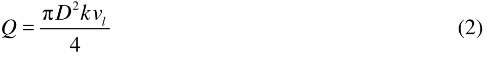
where k is the ratio of the profile average velocity on the pipe cross-section vsto vl

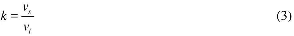
If the k is obtained, we can calculate the volume flow of the pipe. The Industrial AutomationInstrumentation Manual[1]provides the values ofk for the ultrasonic flow meter under the condition that the pipe flow is a laminar or a fully-developed turbulent flow. But there is no appropriate method of calculating k for a transition flow while the Reynolds number is in the range of 2 300-13 800. In many cases, the flow within the ultrasonic flow meter is a transition flow. For example, the volume flow of most household heat meters is less than 0.25 m3/h and the Reynolds number is less than 7 500, in the transition region. The traditional method is to take the transition flow as the turbulent flow to calculatek , which may lead to measurement errors. In order to improve the measurement accuracy of the ultrasonic flow meter, it is necessary to study the transition pipe flow.

The numerical simulation is an important method of studying the flow characteristics in a pipe. The turbulent models based on the Reynolds average, such as the standardk-εand the RNG k-εmodels, are not suitable for simulating the transition flow. The Direct Numerical Simulation (DNS) method can directly solve the Navier-Stokes equations with high accuracy and can simulate all scales of turbulent flows. In recent years, the DNS method has witnessed a rapid development with many good results. It is shown[2-8]that the DNS method can be used to obtain accurately the turbulent flow field. In the numerical simulations of the pipe flows, Wu and Zhang[9]use the spectral method to calculate the turbulent velocity field in a cylindrical coordinate system and study the structure of the turbulence flow within a pipe. Mellibovsky et al.[10]simulates the transitional pipe flow in a long computational domain with the DNS method, and Wu et al.[11]simulates the fully developed turbulent pipe flow at Re =24580. These studies mainly focus on the simulations of the flow structure, and not so much on engineering problems such as the relationship between the linear average velocity vland the profile average velocity vs. In this paper, the DNS method is used to simulate the flow field of a pipe when the Re is 2 600, the velocity and pressure distributions in the pipe are obtained. On this basis, the ratio of the profile average velocity on the pipe crosssection vsto vlis obtained. This study may shed light on how to improve the measurement accuracy of the ultrasonic flow meter, as well as the study of the pipe flow characteristics.

1. Governing equations

The incompressible dimensionless Navier-Stokes equations in cylindrical coordinates are in the following forms:

Continuity equation

Momentum equations

where Ur,Uθand Uzare the dimensionless radial, circumferential and axial velocity components, respectively,tand p are the dimensionless time and pressure, respectively. The friction speed is taken as the characteristic velocity and the pipe diameterD as the characteristic length to obtain the dimensionless equations.

2. Numerical method and computational domain

2.1 Numerical method

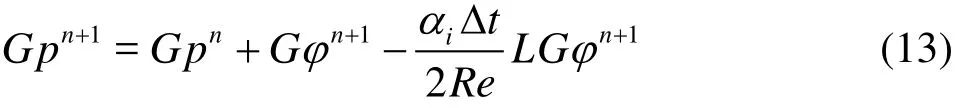
The finite-difference scheme is used to solve the Navier-Stokes equations. The twelfth-order conservative difference scheme is used to discretize the convection term and the central difference scheme is used to discretize the viscous term. The third-order Runge-Kutta scheme combined with the Crank-Nicholson scheme is used to achieve the time discretization, with a time step being divided into three sub-steps and with a pressure correction in each sub-step. The velocity of each sub-step is calculated as:

L is the Laplace operator in a discrete form and D is the discretized divergence operator:

The pressure is calculated from

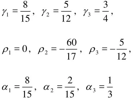
γl,ρland αlare the coefficients in the third-order Runge-Kutta scheme:

2.2 Computational domain and initial conditions

Figure 2 shows the computational domain and meshes. The pipe’s diameterD is 0.04 m and the pipe’s length is4π D . The uniform mesh is adopted in the axial and circumferential directions. The nonuniform mesh is used in the radial direction to refine the grids near the wall. Theoretically, the mesh scale of the DNS should be smaller than the smallest scale of the turbulence-Kolmogorov micro-scaleη. The dimensional analysis shows that the number of nodes in one-dimensional direction is proportional to Re3/4

According to Eq.(14), the number of nodes in the radial, circumferential and axial directions should be 360, 720 and 4 300, respectively, but these node numbers are too large for the computers to handle. Moin and Mahesh[12]shows that the minimum mesh size can be enlarged to 4η-10η, so the number of nodes in the radial, circumferential and axial directions are set to 90, 90 and 600, respectively, which results in a total node number of 4.86×106. The numerical calculations are carried out on a Dell Power Edge C5000 sever, with 24 CPUs and 16G of memory. The parallel computing method is used to realize the numerical simulation and 3 000 iterative steps can be completed in one day.

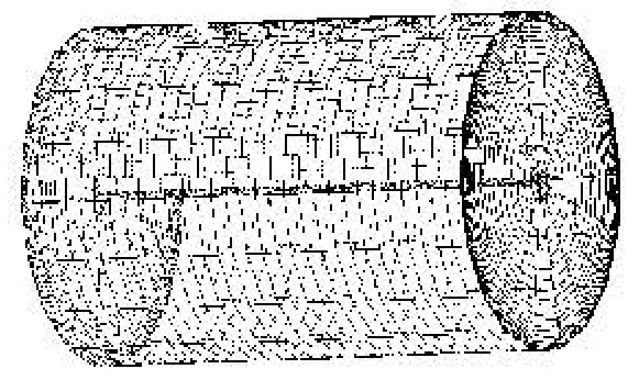
Fig.2 The computation domain and meshes

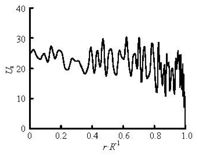
Fig.3 The initialization of velocity

The no-slip boundary condition is adopted in the wall and the periodic boundary condition is set in the axial and circumferential directions. The computational domain is initialized before the start of the calculation. Figure 3 shows the initialization of the velo-city field in the axial direction, the velocity in the axial direction is assigned in accordance with a logarithmic law and a random disturbance is assumed for the velocity field.

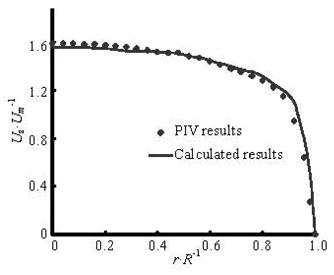
Fig.4 The average velocity profile

Fig.5 The comparison between calculated results and logarithmic law

3. Results and analyses

The pipe flow field is simulated in this paper with the DNS method whenRe is 2 600. The calculated results are saved every 10–3of the dimensionless time after the flow’s full development, so the flow characteristics in the pipe can be statistically analyzed according to the saved results. Figure 4 shows the calculated velocity profile on the pipe cross-section. Umis the average velocity on the pipe cross-section, R is the diameter of the pipe. From Fig.4, it is seen that the velocity profile is consistent with the turbulent flow characteristics in the pipe. Fig.4 also shows the experimental results obtained by the PIV method when the flow is turbulent[13,14]. As shown in Fig.4, the calculated results agree well with experimental results and the pipe flow shows the turbulent characteristics because strong disturbances are applied to the flow field during the initialization. According to the turbulence theory, the velocity profile outside the boundary layer should obey the logarithmic law wherek is 0.4 andC is 5.5 for the pipe flow. Figure 5 shows the comparison between the calculated velocity profile and that of the logarithmic law.

From Fig.5, the velocity profile agrees with the logarithmic law while y+is larger than 30. When y+is less than 30, the flow can be considered to be in the viscous sublayer and the velocity profile obeys the linear law. The velocity profile is not shown in Fig.5 when y+＜30.

Figure 6 shows the turbulence intensity in the axial direction against the radial position. Figure 7 shows the Reynolds stress against the radial position. The distributions of the turbulence intensity and the Reynolds stress shown in Fig.6 and Fig.7 agree with the previous experimental and numerical results[15,16]. Figures 4 to 7 can validate the numerical methods used in this paper.

Fig.6 The turbulence intensity in axial direction

Fig.7 The Reynolds stress distribution

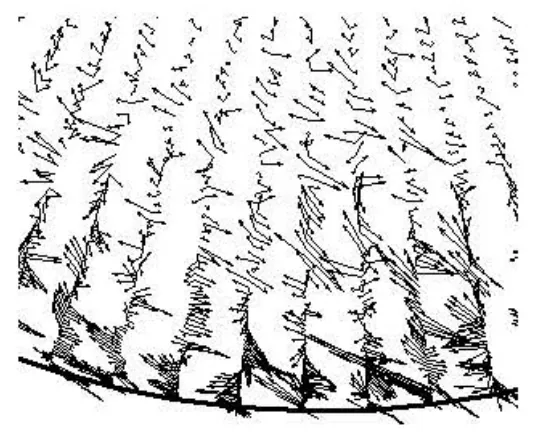
Fig.8 The calculated velocity vector on cross section

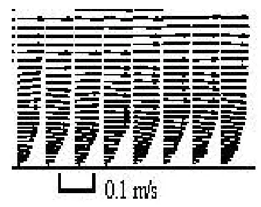
Fig.9 The calculated velocity vector on longitudinal section

Fig.10 The velocity vector in longitudinal direction

Figure 8 and Fig.9 show the calculated velocity vector near the wall on the lateral and longitudinal sections. Figure 10 shows the experimental velocity vector obtained by the PIV method. From Fig.8, a swirl structure can be seen near the wall. The comparison between Fig.9 and Fig.10 shows that the calculated results can match the experimental results and the calculated results can more explicitly show the characteristics of the flow within the boundary layer.

The calculated results show that the direct numerical simulation method with finite-difference schemes can be used to correctly obtain the flow information such as the velocity distribution, and the turbulence intensity. Based on the results of the numerical simulation, the coefficientk of the ultrasonic flow meter (as shown in Fig.1) can be calculated. In this paper, the value ofk obtained by the DNS is 0.892. Ref.[1] suggests that the coefficientk for a turbulent flow can be obtained by the following formula

According to Eq.(16), the coefficientk is 0.919 When the Reynolds number is 2 600, the difference is 3.02%. It shows that the velocity profile of a transition flow is different from that of a turbulent flow and the flow flux obtained with the method for the fully developed turbulent flow will lead to measurement errors for the ultrasonic flow meter.

4. Conclusion

In this paper, a finite-difference scheme for the three-dimensional incompressible flow in the cylindrical coordinates is used to solve the flow field of a pipe when the Reynolds number is 2 600. The third-order Runge-Kutta scheme in combination with the Crank-Nicholson scheme and the twelfth-order conservative finite-difference scheme are used for the solution. The velocity and pressure distributions are obtained by the direct numerical simulation. The comparison between the PIV experimental results and the calculated results shows the validity of the DNS method. On this basis, the ratio of the linear average velocity along the ultrasonic propagation path to the profile average velocity on the pipe cross-section is obtained for an ultrasonic flow meter. It is shown that a large error exists by using the traditional way of using a fully developed turbulence flow to calculatek for a transition flow, and it is important to study the velocity profile for improving the measuring accuracy of the ultrasonic flow meter in the case of a transition flow. The study of this paper sheds some light for improving the measurement accuracy of the ultrasonic flow meter. The next step is to study the velocity profile in the pipe while the Reynolds number is in the range of 2 300-13 800.

[1] THEDITORIAL BOARD INDUSTRIAL AUTOMATION INSTRUMENTATION MANUAL.Industrial Automation Instrumentation Manual[M]. Beijing, China: Mechanical Industry Press, 1988(in Chinese).

[2] SIRISUP S., KARNIADAKIS G. E. and SAELIMB N. et al. DNS and experiments of flow past a wired cylinder at low Reynolds number[J].European Journal ofMechanics B/Fluids,2004, 23(1): 181-188.

[3] GEI Ming-wei, XU Chun-xiao and CUI Gui-xiang. Dirent numerical simulation of flow in a channel with time-dependent wall geometry[J].Applied Mathematics and Mechanics,2010, 31(1): 91-101(in Chinese).

[4] OULD-ROUISS M., REDJEM-SAAD L. and LAURIAT G. Direct numerical simulation of turbulent heat transfer in annuli: Effect of heat flux ratio[J].International Journal of Heat and Fluid Flow,2009, 30(4): 579-589.

[5] YU Bo, WANG Yi and HOU Lei et al. Direct numerical simulation on the drag-reducing flow by surfactant additives at various rheological properties[J].Journal of Engineering Thermophysics,2007, 28(3): 469- 471(in Chinese).

[6] ZHU Zuo-jin, YANG Hong-xing and CHEN Ting-yao. Direct numerical simulation of turbulent flow in a straight square duct an Reynolds number 600[J].Journal ofHydrodynamics,2009, 21(5): 600-607.

[7] LI D., FAN J. andLUO K. et al. Direct numerical simulation of a particle-laden low Reynolds number turbulent round jet[J].International Journal of MultiphaseFlow,2010, 37(6): 539-554.

[8] LI Bu-yang, LIU Nan-sheng and LU Xi-yun. Direct numerical simulation of turbulent heat transfer in a wall normal rotating channel flow[J].Journal of Hydro-dynamics,2006, 18(1): 26-31.

[9] WU Min-wei, ZHANG Zhao-shun. Numerical research on the structures in turbulent pipe flow[J].Journal of Hydrodynamics, Ser. A,2002, 17(3): 334-342(in Chinese).

[10] MELLIBOVSKY M., MESEGUER A. and SCHNEI-DER T. M. et al. Transition in localized pipe flow turbulence[J].Physical review letters,2009, 103(5): 529- 534.

[11] WU X., BALTZER J. R. and ADRIAN R. J. Direct numerical simulation of a30R long turbulent pipe flow at R+=685: Large-and very large-scale motions[J].Journal of Fluid Mechanics,2012, 698: 235- 281.

[12] MOIN P., MAHESH K. Direct numerical simulation: a tool in turbulence research[J].Annual Review of FluidMechanics,1998, 30: 539-578.

[13] LIU Yong-hui, DU Guang-sheng and LIU Li-ping et al. Experimental study of velocity distributions in the transition region of pipes[J].Journal of Hydrodynamics, 2011, 23(5): 643-648.

[14] LIU Yong-hui. Research of characteristics of transition flow in pipes[D]. Doctoral Thesis, Jinan: Shandong University, 2011(in Chinese).

[15] FENG Bin-chun, CUI Gui-xiang and ZHANG Zhaoshun et al. Experimental study of fully developed turbulent pipe flow[J].Acta Mechanica Sinica,2002, 34(2): 156-167.

[16] Van DOORNE C. W. H., WESTERWELL J. Measurement of laminar, transitional and turbulent pipe flow using Stereoscopic-PIV[J].Experiments in Fluids,2007, 42(2): 259-279.

10.1016/S1001-6058(13)60346-7

* Project supported by the National Natural Science Foundation of China (Grant No. 10972123).

Biography: LIU Zheng-gang (1973-), Male, Ph. D., Lecturer

DU Guang-sheng, E-mail: du@sdu.edu.cn