Simulation of wind-driven circulation and temperature in the near-shore region of southern Lake Michigan by using a channelized model*

LIU Lubo

Department of Civil and Geomatics Engineering, Lyles College of Engineering, California State University, Fresno, California 93740, USA

State Key Laboratory of Hydroscience and Engineering, Tsinghua University, Beijing 10084, China, E-mail: llubo@csufresno.edu

FU Xu-dong, WANG Guang-qian

State Key Laboratory of Hydroscience and Engineering, Tsinghua University, Beijing 10084, China

Simulation of wind-driven circulation and temperature in the near-shore region of southern Lake Michigan by using a channelized model*

LIU Lubo

Department of Civil and Geomatics Engineering, Lyles College of Engineering, California State University, Fresno, California 93740, USA

State Key Laboratory of Hydroscience and Engineering, Tsinghua University, Beijing 10084, China, E-mail: llubo@csufresno.edu

FU Xu-dong, WANG Guang-qian

State Key Laboratory of Hydroscience and Engineering, Tsinghua University, Beijing 10084, China

(Received July 3, 2012, Revised Novmber 22, 2012)

To enhance the efficiency of a pathogen forecasting model in the beach areas of southern Lake Michigan and to reduce the computation time, the near-shore current is approximated as a channelized flow parallel to the shorelines in clockwise or anti-clockwise direction within the accuracy tolerance range. A channelized model with a curvilinear boundary can significantly reduce the computation effort, and at the same time achieve a good agreement between the predicted and measured water surface elevations, currents, and water temperatures. The sensitivity analysis results show that the suitable channel width for the near-shore region of southern Lake Michigan should be no less than 10 km. The modeling results of the water temperature are much less sensitive to the channel width than those of the current velocity and the water surface elevation. The modeling results also show a close correlation between the speeds of the wind and the near-shore current. The current may fully respond the wind stress with a time lag of several hours. The correlation may provide an approximate estimation of the lake circulation under some wind conditions for a practical forecasting purpose. More complex wind-current relationships need to be described with a more sophisticated hydrodynamic model. This verified model can be used for the pathogen forecasting in the near-shore regions of southern Lake Michigan in the future.

near-shore, channelized, wind, hydrodynamic model

Introduction

Lake Michigan can serve numerous recreational purposes, such as swimming, fishing, and boating, for millions of people every year. In the near-shore areas, the fragile regions with most frequent human activities, the water quality degradation caused by pathogens and other contaminants attracts more and more attention due to the potential risk to human health. Therefore, the water quality prediction in the near-shore regions is of interest to beach managers and the public. Effort was devoted to maximize the recreational beachmonitoring accuracy and efficiency in recent years. Water samples were generally collected from the shallow water along the shoreline of near-shore regions for routine water quality checks[1].

The effectiveness of a conventional warning system for recreational waters by sampling and labtesting is usually constrained by the long water sampling period and the lengthy lab analysis procedure, and therefore, the warning may be delayed[2]. For example, it usually requires a 24 h incubation period for monitoring Escherichia Coli (EC), a commonly used pathogen indicator, by the experimental analysis. However, people may unintentionally drink or swim in the contaminated water in the meantime. To avoid the delay and to promptly inform the beach goers and protect them from the exposure to waterborne pathogens, mathematical models were widely used as an effective tool to obtain quick forecasting results of hydrodynamic conditions and water quality, and to provide warnings and simulations in time.

A complete pathogen modeling program generally consists of a water quality model for the pathogenic contaminant concentration prediction coupled witha hydrodynamic model for the circulation and the water surface elevation simulation. The fate and transport of pathogens in a water body as Lake Michigan are largely related with its hydrodynamic conditions, including the variations of current velocity, water depth, water surface flocculation, and water temperature affecting the pathogen inactivation and growth. Therefore, a hydrodynamic model that can provide a quantitative description of these parameters is the foundation of the water quality simulation and the accuracy of the pathogen forecasting.

There were extensive modeling studies related with the Great Lakes[3-7]. Some hydrodynamic modeling studies were carried out for Lake Michigan[8,9]. Examples of these models include three-dimensional stratified models[10,11]and two-dimensional depth averaged models[12]. As a part of the whole lake, the nearshore regions exchange momentum, energy and mass with the offshore areas. Hydrodynamic models were used to simulate the near-shore flow fields that are both complex and varying with time. In most nearshore hydrodynamic models, focuses were on solving the complex interactions between the near-shore and offshore regions. These sophisticated models were applied to delineate the circulation and the temperature by meshing the entire water body and refining the local near-shore domain. However, to cover a large area in a mathematical model requires a large amount of computation in the same detail consideration and the accuracy requirement. Therefore, such an approach could be very demanding from a forecasting point of view due to the excessive computational amount notwithstanding the ever enhanced computer capacities these days. Some studies[12]show that the wind-induced long-shore currents flow parallel to the shoreline and are strongest in the near-shore zone. Comparing to the flows in the cross-shoreline direction, the currents along the shoreline overwhelmingly predominate the near-shore circulation. Therefore, to enhance the modeling efficiency and to reduce the computation time, the near-shore current within the lake wide circulation might be approximated as a channelized flow parallel to the shorelines in clockwise or anti-clockwise direction within an acceptable accuracy tolerance range. The exchanges of the mass and the momentum in the cross-shore direction are assumed to exist only within the channel. A modeling domain with such boundary conditions is simplified as a closed open channel along the shoreline of Lake Michigan. From the water forecasting point of view, the significant reduction of the offshore area as well as the mesh number, and thus the computation amount can substantially reduce the time to obtain the modeling results, therefore to promptly keep people away from the pathogen contaminated beach water. It can also guide the managers to take corresponding measures in time to reduce the risk to human health.

Based on the long-shore-dominant assumption, this research is a continuation of previous modeling investigations of pathogen inactivation in the nearshores of Lake Michigan[12]. The previous 2 d averaged water depth model were verified and calibrated with the data collected in a 34 d period (between Julian days 194 and 227 of 2006). The model with a meshed full-lake was successfully applied to the inactivation investigation of EC and enterococci (ENT) in southern Lake Michigan. However, it takes about 3.5 h with the lake wide hydrodynamic model to simulate a one-month circulation of Lake Michigan, not a very long predictive period. The hydrodynamic calculation is relatively time-consuming and not very effective from a water forecasting point of view. In addition, a long computing process is a fact not desirable for simulating numerous scenarios for in-depth parametric sensitivity analysis as well. To solve this problem, a new channelized model of treating the near-shore region as an open channel is developed to enhance the modeling efficiency for the forecasting and investigation of hydrodynamics and water quality of Lake Michigan. In this study, a 55 d data set (from Julian day 173 to 227) is used for the hydrodynamic and water temperature verification and calibration. The sensitivity of the channel width on the currents and the temperature in the near-shore of Lake Michigan is studied with the channelized model. The model is also used to investigate the correlations between the wind and the lake current. This quick response model will be further used as the basis of the parametric sensitivity analysis of the pathogen fate and transport in Lake Michigan in the future.

1. Mathematical models

The model system consists of two components: a hydrodynamic model for the lake circulation simulation coupled with a transport model for the temperature modeling.

1.1 Model mesh

To delineate the complex shoreline of Lake Michigan accurately, a finite-element model is developed by using triangular and quadrilateral isoparametric elements. Six and eight nodes are used to define these elements, respectively. In each case, three (for triangular element) or four (for quadrilateral element) nodes are placed at the vertices and on the sides, respectively. The exact position of the mid-side node determines the curved shape of the side. Within an element, the quadratic approximations are used to represent the velocities, the water depths and the temperatures. The non-uniform mesh resolution is between 30 m and 3 km covering all near-shore regions along the shoreline of Lake Michigan.

1.2 Hydrodynamic model

Since the primary interest of this research is in the near-shore regions where the water depths are shallow, a vertically integrated hydrodynamic model is used with the finite element scheme RMA10[13]to describe the wind-driven circulation and the water temperature. The vertical integrated hydrodynamic equations in x and y directions are

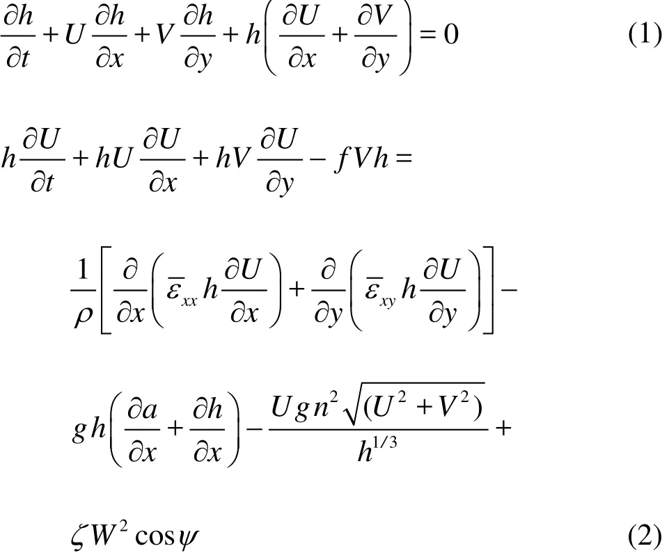
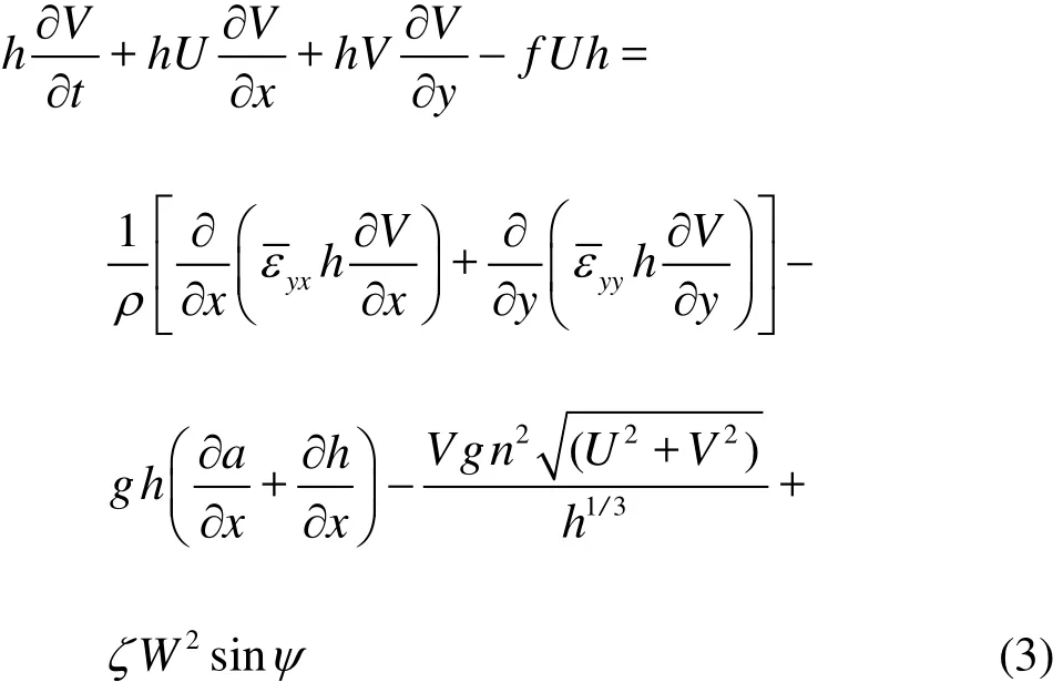
whereU,V are the depth-averaged velocities inx, y directions,h is the water depth and a is the bottom surface elevation,W is the wind velocity, ψis the wind direction,ζis an empirical wind coefficient,f is the Coriolis parameter, and g is the gravity acceleration.n denotes the Manning’s roughness coefficient, andis the depth-averaged eddy viscosity. In the momentum Eqs.(2) and (3),is described by using the Smagorinsky eddy parameterization as

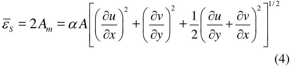
where αDis a correction constant,V is the velocity vector and LSis the characteristic length scale, which is the element size in this model.

1.3 Temperature model

The temperature plays an important role in the pathogen simulation and forecasting because the inactivation of pathogens is very sensitive to the water temperature. Therefore, the temperature model is another major aspect of a pathogen forecasting model. The water temperature in the near-shore region of a fresh water body is primarily determined by loadings from tributaries as well as the radioactive exchange with the overlying atmosphere. In this research, a full atmospheric heat budget at the water surface water temperature is included. The model considers the heat flux forcing at the surface, and the zero heat flux at the bottom. To be consistent with the future pathogen transport model, the governing equations of the temperature and the pathogen concentrations are as follows[15]

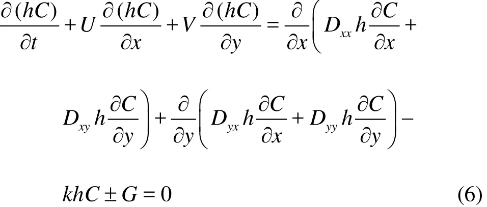
where C is the depth-averaged temperature or pathogen concentration,Dxx,Dxy,Dyy,Dyxare the depth-averaged dispersion and turbulent diffusion coefficients in different directions, andG denotes a general source or sink term and it can be expressed for the temperature as

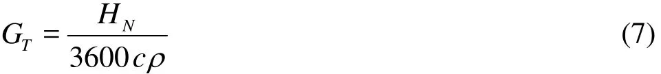
Table 1 Model parameter list

where c is the heat content of the water,ρis the density, and HNis the net heat flux passing the air water interface, which is determined as

where HSNis the net short-wave influx,HANis the net long-wave influx,HBis the long-wave back radiation,HEis the conductive flux, and HCis the evaporative flux. The transport Eq.(6) is coupled with the hydrodynamic model and is solved by using the RMA11[15]for the temperature determination. Details of these different fluxes and the ranges of parameters involved were described by Martin and McCutcheon. The meterological data needed to run the temperature model for the determination of each influx in Eq.(8) include the atmospheric pressure, the cloudiness, the bulb temperatures, the dust attenuation, the solar radiation rate, the water temperature and the wind velocity (Table 1).

1.4 Boundary and initial conditions

To specify the initial conditions for the model, it is assumed that the lake is at rest at time t =0. The initial temperature at each node is determined by interpolation of the observed data collected at the meteorological stations in Fig.2. The boundary conditions for the hydrodynamic model include the no leakage condition across the surface and the bottom, the wind stress and the zero pressure at the free water surface, and the drag stress on the bottom of the lake. In the temperature model, the boundary conditions include the observed temperature variations at the outfalls of the tributaries and the heat exchange between the lake surface and the atmosphere.

1.5 Model parameter specification

The parameters used as the input of the model are listed in the alphabetic order in Table 1. Different time steps (6 h and 5 min) are used in this modeling investigation. The meteorological data (such as the air pressure and the wind velocity) vary with time and they are the dynamic inputs to the model. The values of these dynamic parameters listed in Table 1 are the averaged values. In the convergence test, 0.1% and 0.05% are set as the convergence criteria for the current velocities/temperature and the WSE at each iteration within a dynamic step (Table 1).

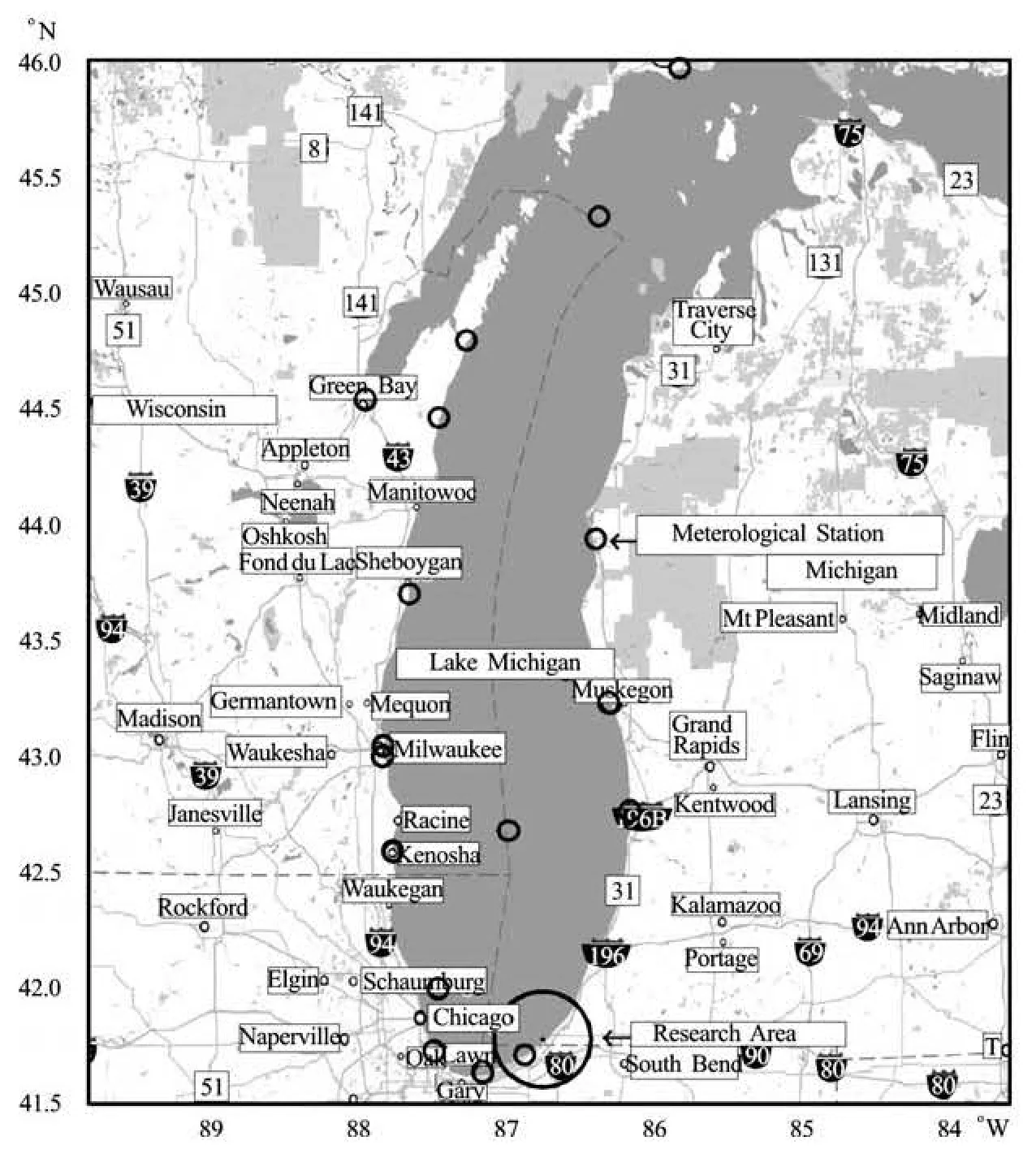
Fig.1 Google road map of Lake Michigan and the research area

2. Investigation site and observation data

2.1 Site description

This modeling research mainly focuses on an approximately 100 km-long shoreline within the nearshore region of southern Lake Michigan (Fig.1). There are four primary tributaries flowing into the investigation domain, including Trail Creek (TC) at Michigan City Harbor (USGS 04095380), Kintzele Ditch (KD) at Michigan City nearby, Burns Ditch (BD, USGS 04095090), and Indiana Harbor Canal (IHC) at East Chicago (Figs.2(e) and 2(f)). Comparing to other neighboring creeks with much less discharge, these tributaries not only contribute the water flux but also act as point sources of pathogens and other pollutants to the domain of interest (Fig.2(f)), and thus are mainly considered in this model. The Mt. Baldy (MB) Beach between KD and TC and the Central Avenue (CA) are chosen as the target beach locations of the pathogenic contaminant study in the near-shore area (Fig.2(f)). The hydrodynamic investigation in this study serves as the foundation of the pathogen forecasting at these two recreational beaches for the beach management.

2.2 Observation data

The major factors considered in the hydrodynamic model include the lake bathymetry, the depiction of lake shorelines, the wind speed and direction, the hydrological flows from tributaries, and the water temperature. The meteorological data and the bathymetry data are collected at different meteorological stations of Lake Michigan (Fig.2) as the model input. The measured Water Surface Elevations (WSEs), the velocities of the current circulation, and the water temperatures are used for the model verification and calibration during the modeling period.

2.2.1 Input meteorological data

As the inputs of the models, the hourly meteorological data including the wind speed and direction, the air temperature, the dew point temperatures, the air pressure, the sunlight insolation, and the evaporation rate are obtained from seven stations of the NOAA National Climatic Data Center (NCDC) and two buoys of NOAA National Data Buoy Center (NDBC) (Figs.1 and 2(e)). These stations include Ludington and Muskegon in Michigan, Michigan City in Indiana, Calumet Harbor and Chicago in Illinois,Sheboygan and Milwaukee in Wisconsin, and two NDBC buoys (45002 and 45007) in Lake Michigan.

Fig.2 Finite element meshes with different channel widths

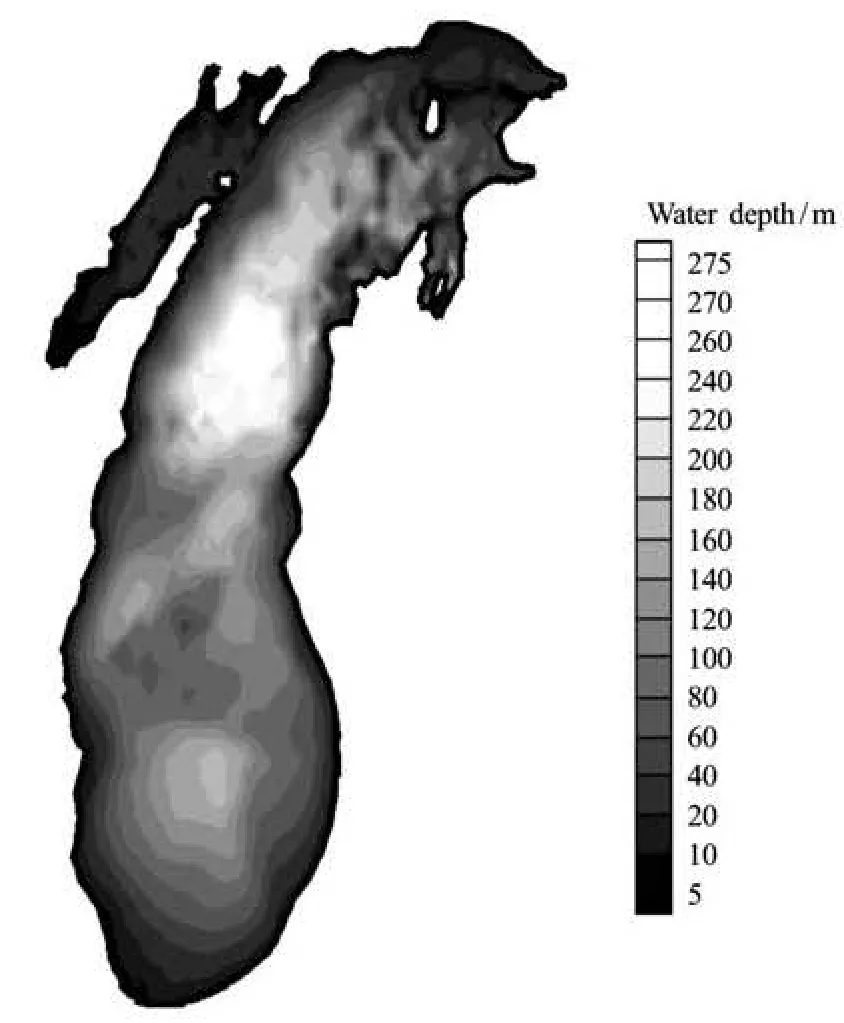
Fig.3 Bathymetry contour of Lake Michigan

2.2.2 Bathymetry data

The circulation in Lake Michigan is driven primarily by the wind, the Earth’s rotation, the lake basin topography, and the vertical density structure[16]. The lake circulation largely depends on the lake bathymetric scenario. The southern part of Lake Michigan is a gradual sloped conical depression with a maximum depth of around 178 m in the center, and the water depth in the near-shore zone is generally less than 40 m (Fig.3) and within several meters in the recreational beach area. In this research, the bathymetry data with a resolution of three arc-seconds shown in Fig.3 are collected from the NOAA National Geophysical Data Center (NGDC)

2.2.3 Model calibration data

The data of the current velocities and the WSEs with 6 h time increment at BD and GB for model verification and calibration are acquired from the Center for Operational Oceanographic Products and Services(COOPS) and the NDBC of NOAA. The data of the water temperatures collected at MB and CA are used for the temperature model calibration.

3. Results and discussions

The near-shore regions of Lake Michigan are delineated as a looped open channel with different widths (5 km, 10 km and 15 km) and their modeling results are compared with those of a full-lake mesh. Figure 2 shows the corresponding meshes, the locations of the observation stations, and the investigation domain. The modeling period is 55 d (between Julian day 173 and 227 of 2004), as is consistent with the data collection period in this study and 20 d longer than the previous study[12].

Fig.4 Discharges to southern Lake Michigan from four tributaries

Fig.5 Comparisons between the results of modeling with various meshes and the observed data

Fig.6 The current velocity vectors in MB near-shore region

3.1 Model calibration

The extensive tests with the observed currents, the water level fluctuations, and the water temperature variation distributions were carried out during the model development. As the flow boundary conditions, the temporal discharges of the four main tributaries flowing into southern Lake Michigan are shown in Fig.4. Even though small tributaries as TC and KD do not provide much flow (less than 5 m3/s in the investigation period), they are considered in this model dueto their significant impact on the pathogen levels at the nearby near-shore region as point sources. The outfalls of TC and KD are the closest point sources of pathogens to the target beaches (MB and CA) in the research area. BD is the most discharged creek and is located much farther away from MB and CA as compared to TC and KD.

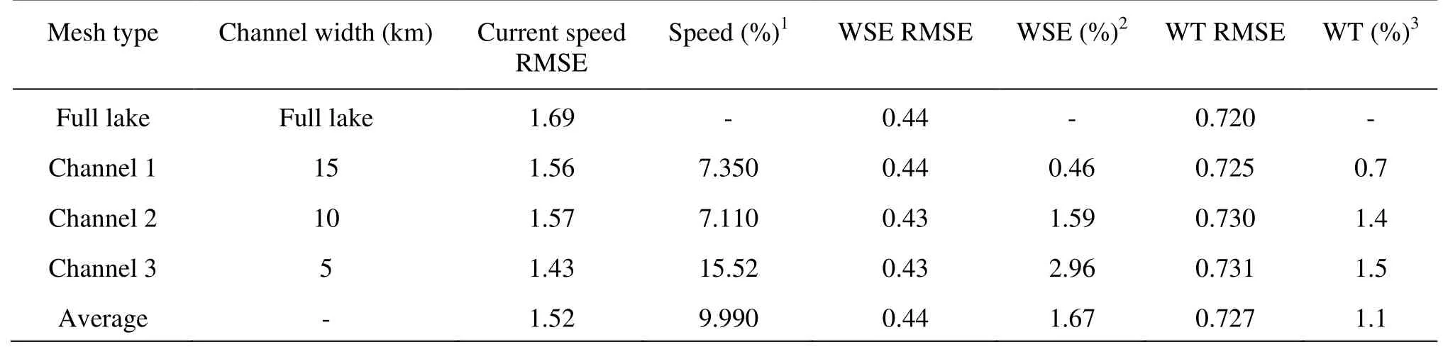
Table 2 RMSE of different meshes

The developed hydrodynamic model is calibrated by using the observed current speed data obtained from a 1 200 KHz Acoustic Doppler Current Profiler (ADCP) at BD (July 2-August 14) and the monitored WSEs at Green Bay (GB) station of Lake Michigan (June 21-August 14). Figure 5 shows the comparisons between the modeling results of the current speed and the WSE from four different meshes in Fig.2 and the observed data. The simulated current speeds are of the same order of magnitude as the data and the model fairly describes the current speed (Fig.5(a)). The discrepancies between the data and the modeling speeds come mainly from the lack of high resolution coastline and bathymetry data, and partially from averaging of the ADCP data as well. Both the modeling and observed WSEs vary in consistent trends and the model can capture most peak and trough values of the data (Fig.5(b)). The current velocity fields obtained from the hydrodynamic model (Figs.5 and 6) are generally found to be consistent with the known circulation patterns in southern Lake Michigan. In overall, the model can describe the observed data quite accurately, and can provide a reasonable hydrodynamic simulation.

3.2 Sensitivity of channel width

The modeling results obtained from different channelized meshes (Channels 1, 2 and 3 in Table 2), are compared with those from a full-lake mesh (Fig.2(d)). The comparisons are shown in Fig.5. All of these meshes have exactly the same resolutions in the near-shore region, and the only difference between any two of them is the additional elements in wider channels. Figure 5 shows quite close modeling results obtained from different meshes. Slightly higher current speeds and lower WSEs are observed as the channel width increases. The narrower channel must elevate its WSE to a higher level to contain the same amount of additional water from tributaries, and thus leads to a lower current speed. In near shore regions, the shoreline acts as a lateral constraint on the water movement and forces the current to move nearly parallel to the shoreline. The offshore current may occur at some places far from the shoreline (Fig.6). Figure 6 shows the current velocity field at different instants by using Channel 1 mesh (15 km wide channel, Table 2).

The application of the channelized model can save the modeling time significantly, and the narrower channel used means less computation amount. However, the sensitivity of the width of the channel should be checked before it is applied to a practical forecasting or other hydrodynamic investigations. The sensitivity investigation is carried out on the basis of Root Mean Squares Error (RSME) analysis. The un-normalized RSME for comparisons between the observed data and the modeling results of each channelized mesh is formulated as

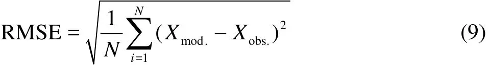
where Xmod.and Xobs.are the modeling and observed speeds/WSEs, respectively, and N is the number of observations.

The current speeds at BD and WSEs at GB are used for the RSME comparisons between different channelized meshes. The west-east distance of southern Lake Michigan is around 130 km. Comparing to the full lake mesh (Fig.2(d)), the averaging variation of the current speed RSMEs obtained from Channels 1, 2 and 3 is within 10% (9.99%, Table 2). The RSME values of WSE of different meshes are quite close to 0.44 and 0.43 and the averaging RSME variation is 1.67%, indicating little WSE change resulted from different widths of channels. A 15.51% difference of the current speed RSME from the full-lakemesh is observed with the 5 km channel mesh. The increase of the channel width to 10 km leads to a 7.11% change, and little further change of 7.69% occurs for a 15 km mesh. Channels 1 and 2 have very close RSMEs (1.56 and 1.57 for the current speed, 0.44 and 0.43 for WSE), even lower than those obtained from the full lake mesh (1.69 and 0.44). As a result, the hydrodynamic conditions are rather stable and not sensitive to the channel width within a certain range (wider than 5 km-10 km), and a several-km open channel flow can be used to replace the more than one hundred km wide Lake Michigan to fairly describe the hydrodynamic scenario in the near-shore region.

Fig.7(a) RMSE changes with different channel widths

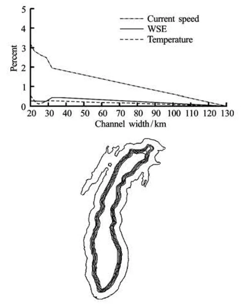
Fig.7(b) Difference percentage between a channelized mesh and the full mesh model with various channel widths

In addition to the three meshes used in this model, five more channelized meshes were also tested by changing channel widths from 20 km to 32 km with an increment of 3 km to check the model’s sensitivity to channel width and their corresponding convergence. Figure 7 presents the boundaries of the five additional meshes and their RMSEs compared with the observed data. Even though Fig.7(a) shows a slightly mounting trend of RMSEs as the channel width increases to a full lake (130 km wide), one should not conclude that a narrow channel may better describe data than the full lake mesh due to the limitation of observed data. Figure 7(b) shows the comparisons of RMSEs between channelized meshes with different widths and the full lake mesh. The wider channel results in the less difference percentage from those of the full lake mesh, which indicates that the modeling result converges to the full lake scenario as the width increases to the width of the whole lake.

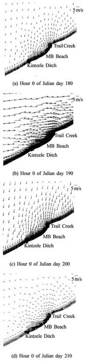
Fig.8 Wind velocity vectors in MB near-shore region

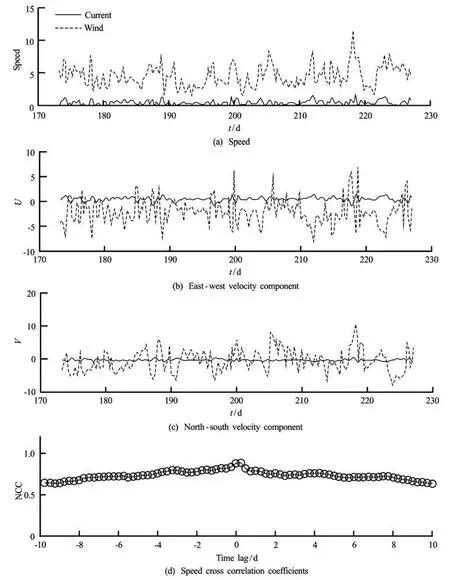
Fig.9 Comparisons and correlations between wind and current at Green Bay

The sensitivity analysis of channel width implies that the channels with certain widths are quite comparable with the full lake mesh. Wider than 20 km, a channelized model may cause much smaller difference from the full lake mesh: less than 0.5% for the WSEs and the temperature and 3% for the circulation speed. If a channelized mesh is adopted, the relative sacrifice of accuracy can be compensated by the advantage of a much faster computation speed, and therefore, a much more prompt prediction, to be acceptable from the practical forecasting point of view.

3.3 Wind stress

In a lake wide scale, the water circulation is mainly driven by the rotation of the earth (Coriolis force), the density gradient and the surface shearing stress such as the wind stress. During the unstratified season as the modeling period (July and August) in this research, the favorite time to most beach-goers, the vertical density structure impacts little on the current of the near-shore shallow water and the thermocline is absent. Thus, the wind action may penetrate deeper into the water column than in other seasons and plays a predominant driving role for the currents.

In the model, the time-dependent wind stress is used. The initial conditions of the water temperature and the wind boundary conditions are obtained by interpolating data with the Inverse Distance Weighting(IDW) method from the metrological stations (small circles in Figs.1 and 2(e)) all over the entire lake. The wind data originally measured at different heights at these stations are converted to those at a common 10 m height as

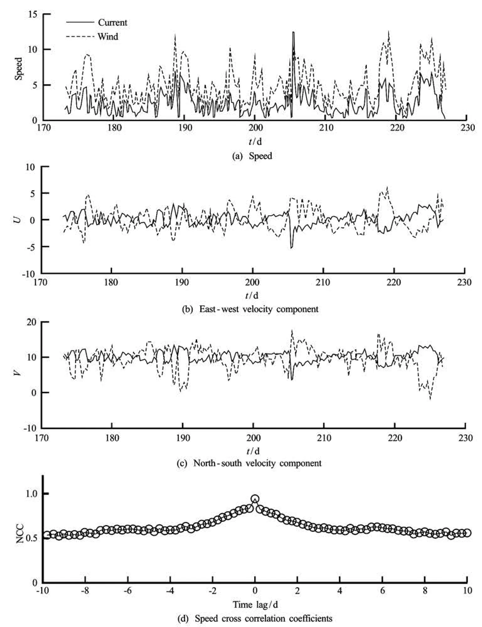
Fig.10 Comparisons and correlations between wind and current at MB Beach

where K (=0.4)is the von Karman constant,z0is the desired height, which is 10 m in this model,z is the actual measurement height,U is the corrected wind velocity with height z0, and U*is the friction velocity.

Figures 6 and 8 show the current circulation and the corresponding wind fields in the investigation domain at four different instants during the investigation period using Channel 1 mesh. The cross-shore current is minor and only occurs in offshore regions and the alongshore current component is predominant in the investigated near-shore region, as is consistent with the characteristics of the near-shore processes[17]. Less obvious correlations between the wind and the current distributions are observed from the vector field comparisons. However, the speeds of the wind and the current show a consistent variation at the same modeling moments. For example, relatively high and lowcurrent speeds at hour 0 of day 190 (Fig.6(b)) and hour 0 of 210 (Fig.6(d)), respectively, correspond high and low wind speeds at the same instants (Figs.8(b) and 8(d)), even though the directions are not necessarily consistent. To further investigate the correlations between the wind and the current, the cross-correlation is analyzed by examining the magnitude and the temporal distributions of their correlation coefficients. The normalized cross correlation between the wind and the current is defined as

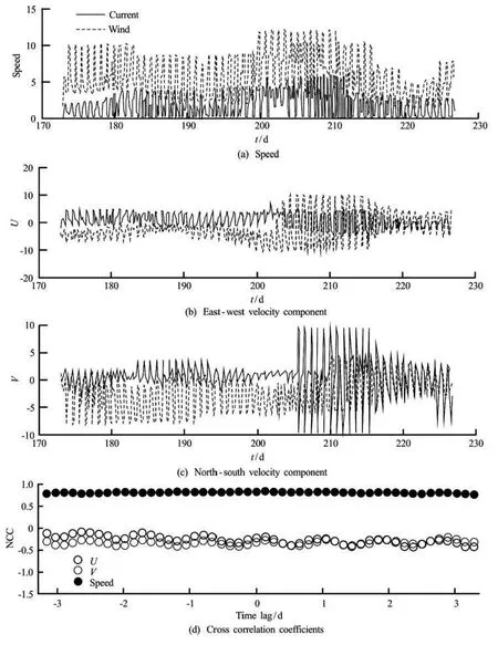
Fig.11 Comparisons and correlations between wind and current at MB beach with 5 min time step

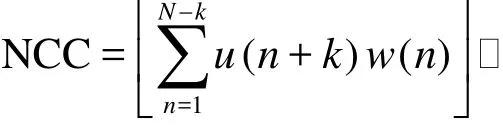
where NCC is the normalized cross correlation function, which takes a value between –1 and 1,u( i) and w( i )are the current velocity and the wind velocity at the ith time step, respectively,N is the number of modeling data,k is the number of time lags.

The correlations between the wind and the lake current are investigated for the near-shore regions in both southern (Center of MB in Fig.10) and northern

(GB in Fig.9) Lake Michigan. The comparisons of the speed and velocity components along north-south (V) and east-west directions (U) between the observed wind and the simulated current are shown in (a), (b), and (c) of Figs.9 and 10, respectively. With a different magnitude, the simulated current speeds at the nearshore regions consistently vary with the observed wind, the primary driving factor of the circulation (Figs.9(a) and 10(a)). Their variations are almost synchronous with a 6 h time step used in the model. The best cross correlation NCC of the speeds is 0.95 without time lag at MB, and 0.8847 with less than one time lag (equivalent to 6 h) at GB. Since the time step used in this model is 6 h, in accordance with the minimum time interval of the observed data, the correlations within a time lag (less than 6 h) between the wind and the current may not be sufficiently reflected. Therefore, the correlation with a much finer time step (5 min) is tested and the results are graphically shown in Fig.11. The maximum NCC values with their corresponding time lags ofU,V and the speed are listed in Table 3. For the new time step, the best speed NCC at MB is 0.83 in the scenario of a 3 h lagged current, which indicates that it will take 3 h for the lake circulation to fully respond the wind stress in the nearshore region. The best speed NCC at GB is 0.9 and the time lag to the wind is around 7 h. Comparing to the 6 h modeling results, the different NCC values are mainly due to the errors caused by the interpolation of the observed wind data to a 5 min interval series from a data set with hourly frequency.

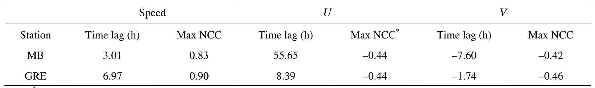
Table 3 Cross correlation coefficients of current and wind velocities (time step is 5 min)

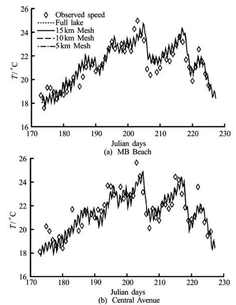
Fig.12 Temperature comparison between modeling results and observed data

The comparable correlations to the wind-current speeds are not observed for the velocity directions of the wind and the current, represented by the velocity componentsU,V in east-west (Figs.9(b), 10(b) and 11(b)) and north-south (Figs.9(c), 10(c), 11(c)) directions, respectively. With a 5 min time step, the absolute values of the best correlation ofU andV are both below 0.5 (Fig.11 and Table 3). Thus, the straightforward relationship between the directions of the current and the wind is not found due to the complex wind-driven hydrodynamic condition.

3.4 Water temperature modeling

The water temperature significantly impacts the pathogen level by changing its inactivation rate related sunlight insolation and sedimentation[12]. The fate and the transport of pathogens and other contaminants are sensitive to their surrounding temperature. Therefore, besides an effective hydrodynamic model, a temperature model is also a key component for a model system to accurately simulate and predict the pathogen levels. The observed water temperatures at the seven observation stations shown in Fig.2(a) are interpolated to the finite-element mesh to create an initial temperature condition for the thermal simulation. The simulated temperatures are compared with the monitored data collected at MB and CA. The modeling results can well match the observed data (Fig.12). Besides the advection and the dispersion in Eq.(6), the water temperature in the model is also dominated by the local heat budget (Eqs.(7) and (8)), which are the same for different meshes. Therefore, the simulated temperatures of four meshes are very close to each other, hardly distinguishable graphically in Fig.12. The changes of RMSE of different channelized meshes from those ofthe full lake mesh are all not greater than 1.5% (Table 2). Very little temperature difference exists among different meshes due to the variation caused by the slight change of the dispersion and the advection with different channel widths.

The comparisons between the observed and simulated temperatures show that the vertically integrated model with a narrow channel width can describe the transport mechanism of the advection and the dispersion reasonably well. To simulate the 55 d period, the computation time using a 10 km (Channel 2) mesh is about 1/7 of the time consumed with the full lake mesh under the same computational condition. The channelized finite-element models of the near-shore hydrodynamics coupled with a temperature model can be used for a quick forecasting of pathogens and other contaminants in the future.

4. Conclusion

In summary, with the channelized model with the curvilinear boundary, a good agreement is achieved between the predicted and measured water surface elevations, currents, and water temperatures. Comparing to the traditional near-shore hydrodynamic model of Lake Michigan, the channelized model can substantially reduce the computational time and can be effectively used for forecasting and in-depth investigation. The sensitivity analysis results show that the suitable channel width for the near-shore region of southern Lake Michigan should be no less than 10 km. Out of this range, the narrower channel may lead to a higher discrepancy from the results of the full lake mesh by changing the current speeds. The modeling results of the water temperature are much less sensitive to the channel width than the current velocity and the water surface elevation. The model is applied to investigate the correlations between the wind and the current of Lake Michigan. The modeling investigation results indicate a close correlation between the speeds of the wind and the near-shore current. The near-shore current may fully respond the wind stress with a time lag of several hours. The correlation may provide an approximate estimation of the lake circulation under a certain wind condition. Their more complex relationships involving the velocity directions, the spatial distribution, etc. need to be described with a more sophisticated hydrodynamic model. This model will be used for the pathogen forecasting in the future.

Acknowledgements

This work was supported by the State key Laboratory of Hydroscience and Engineering of Tsinghua University (Grant Nos. Sklhse-2007-B-03, 2011-KY-4). The support is also from Dr. Panikumar Mantha of the NOAA Center of Excellence for Great Lakes and Michigan State University, and USGS for the monitoring date.

[1] GRANT S. B., SANDERS B. F. Beach boundary layer: A framework for addressing recreational water quality impairment at enclosed beaches[J].EnvironmentalScience and Technology,2010, 44(23): 8804-8813.

[2] NATIONAL RESEARCH COUNCIL (U.S.). COMMITTEE ON INDICATORS FOR WATERBORNE PATHOGENS.Indicators for waterborne pathogens[M]. Washington DC, USA: National Academies Press, 2004.

[3] THOMPSON A., GUO Y. and MOIN S. Uncertainty analysis of a two-dimensional hydrodynamic model[J].Journal ofGreat Lakes Research,2008, 34(3): 472- 484.

[4] ATKINSON J. F., EDWARDS W. J. and FENG Y. Physical measurements and nearshore nested hydrodynamic modeling for Lake Ontario nearshore nutrient study[J].Journal of Great Lakes Research,2012, 38(4): 184-193.

[5] LEON L. F., SMITH R. E. H. and HIPSEY M. R. et al. Application of a 3D hydrodynamic-biological model for seasonal and spatial dynamics of water quality and phytoplankton in Lake Erie[J].Journal of Great LakesResearch,2011, 37(1): 41-53.

[6] SHENG J., RAO Y. R. Circulation and thermal structure in Lake Huron and Georgian Bay: Application of a nested-grid hydrodynamic model[J].ContinentalShelf Research,2006, 26(12-13): 1496-1518.

[7] HALL S. R., PAULIUKONIS N. K. and MILLS E. L. et al. A comparison of total phosphorus, chlorophyll a and zooplankton in embayments, nearshore, and offshore habitats of Lake Ontario[J].Journal of GreatLakes Research,2003, 29(1): 54-69.

[8] CHEN C., JI R. and SCHWAB D. J. et al. A model study of the coupled biological and physical dynamics in Lake Michigan[J].Ecological Modelling,2002, 152(2-3): 145-168.

[9] TOMLINSON L. M., AUER M. T. and BOOTSMA H. A. et al. The Great Lakes Cladophora model: Development, testing, and application to Lake Michigan[J].Journal of Great Lakes Research,2010, 36(2): 287- 297.

[10] BELETSKY D., SCHWAB D. J. and ROEBBER P. J. et al. Modeling wind-driven circulation during the March 1998 sediment resuspension event in Lake Michigan[J].Journal of Geophysical Research,2003, 108(C2): 3038.

[11] THUPAKI P., PHANIKUMAR M. S. and BELETSKY D. et al. Budget analysis of Escherichia coli at a southern Lake Michigan beach[J].EnvironmentalScience and Technology,2009, 44(3): 1010-1016.

[12] LIU L., PHANIKUMAR M. S. and MOLLOY S. L. et al. Modeling the transport and inactivation of E. coli and enterococci in the near-shore region of Lake Michigan[J].Environmental Science and Technology,2006, 40(16): 5022-5028.

[13] KING I. P.RMA-10 user guide-A finite element model for three-dimensional density stratified flow[M]. Pymble, New South Wales, Australia: Resou- rce Moedlling Associates, 2000.

[14] HOLLAND P. R., KAY A. and BOTTE V. Numericalmodelling of the thermal bar and its ecological consequences in a river-dominated lake[J].Journal ofMarine Systems,2003, 43(1): 61-81.

[15] KING I. P.RMA-11 user guide-A three-dimensional finite element model for water quality in estuaries and stream[M]. Pymble, New South Wales, Australia: Resource Moedlling Associates, 2004.

[16] RAO Y. R., MCCORMICK M. J. and MURTHY C. R. Circulation during winter and northerly storm events in southern Lake Michigan[J].Journal of Geophysical Research,2004, 109(C1): C01010.

[17] GRANT S. B., KIM J. H. and JONES B. H. et al. Surf zone entrainment, along-shore transport, and human health implications of pollution from tidal outlets[J].Journal of Geophysical Research,2005, 110(C10): C01010.

10.1016/S1001-6058(13)60343-1

* Biography: LIU Lubo (1972-), Male, Ph. D., Assistant Professor