Mapping soil organic matter in cultivated land based on multi-year composite images on monthly time scales

Jie Song ,Dongsheng Yu # ,Siwei Wang ,Yanhe Zhao ,Xin Wang,Lixia MaJiangang Li

1 State Key Laboratory of Soil and Sustainable Agriculture,Institute of Soil Science,Chinese Academy of Sciences,Nanjing 210008,China

2 Agricultural and Rural Bureau of Luanping County,Luanping 068250,China

3 Chinese Academy of Sciences University,Beijing 100049,China

Abstract Rapid and accurate acquisition of soil organic matter (SOM) information in cultivated land is important for sustainable agricultural development and carbon balance management.This study proposed a novel approach to predict SOM with high accuracy using multiyear synthetic remote sensing variables on a monthly scale.We obtained 12 monthly synthetic Sentinel-2 images covering the study area from 2016 to 2021 through the Google Earth Engine (GEE) platform,and reflectance bands and vegetation indices were extracted from these composite images.Then the random forest (RF),support vector machine (SVM) and gradient boosting regression tree (GBRT) models were tested to investigate the difference in SOM prediction accuracy under different combinations of monthly synthetic variables.Results showed that firstly,all monthly synthetic spectral bands of Sentinel-2 showed a significant correlation with SOM (P＜0.05) for the months of January,March,April,October,and November.Secondly,in terms of single-monthly composite variables,the prediction accuracy was relatively poor,with the highest R2 value of 0.36 being observed in January.When monthly synthetic environmental variables were grouped in accordance with the four quarters of the year,the first quarter and the fourth quarter showed good performance,and any combination of three quarters was similar in estimation accuracy.The overall best performance was observed when all monthly synthetic variables were incorporated into the models.Thirdly,among the three models compared,the RF model was consistently more accurate than the SVM and GBRT models,achieving an R2 value of 0.56.Except for band 12 in December,the importance of the remaining bands did not exhibit significant differences.This research offers a new attempt to map SOM with high accuracy and fine spatial resolution based on monthly synthetic Sentinel-2 images.

Keywords: soil organic matter,Sentinel-2,monthly synthetic images,machine learning model,spatial prediction

1.lntroduction

Soil organic matter (SOM) plays a crucial role in assessing soil fertility and quality (Seelyet al.2010;Bolton and Friedl 2013),and its spatial distribution affects soil nutrient supply,soil structure and soil ecological function (Yuet al.2014;Laiet al.2021).SOM in cultivated land exhibits significant spatial variability due to agricultural practices and accurately mapping SOM with high spatial resolution is vital for proper management of soil quality and sustainability in agriculture.

Currently,there are two common approaches for mapping the distribution of SOM.One is the use of a geostatistical model,but these always require a large number of sampling points to achieve high prediction accuracy and cannot effectively describe the spatial variability over large geographical areas (Webster and Oliver 2010).The other is the use of remote sensing images to predict the spatial distribution of SOM.Previous studies have shown a remarkable correlation between SOM and soil spectral reflectance,particularly in the near-infrared (NIR,700-2,500 nm) and visible (VIS,400-700 nm) wavelengths (Wanget al.2018).Commonly used multispectral satellites,such as Landsat,Sentinel-2 and MODIS offer open access to images that align with the optimal wavelengths for assessing SOM (Shonket al.1991;Hamzehpouret al.2019;Chenet al.2022).The Sentinel-2 mission,consisting of two satellites (Sentinel-2A and Sentinel-2B),is particularly valuable for SOM mapping.Sentinel-2 provides time series images with high revisit frequency (minimum 5 days global revisittime).Further,it offers high spatial resolution images (ranging from 10 to 60 m) and has small errors in system atmospheric correction (Heet al.2021).In addition,the Sentinel-2 spectral bands span across the visible and near-infrared/short-wavelength infrared (VNIR/SWIR) region,including two SWIR bands at around 1,600 and 2,200 nm,which are known to be highly sensitive to variations in SOM (Ben-Doret al.1997).At present,Sentinel-2 has been extensively applied to estimate the spatial variability of SOM.For example,Vaudouret al.(2019) demonstrated the effectiveness of Sentinel-2A images in predicting eight common soil properties in temperate and Mediterranean regions.Guoet al.(2021) acquired the normalized difference vegetation index (NDVI) from time series images from satellites including Sentinel-2,Gaofen (GF) 1,and Landsat 8 to predict SOC,and found that SOC estimations using Sentinel-2 data exhibited superior accuracy compared to the other satellite sources.

The spectral reflectance of single-day satellite images can be influenced by a great deal of interfering factors,such as surface vegetation cover,soil water content,surface roughness and clouds and shadows (Chabrillatet al.2019).To mitigate this limitation,researchers have worked on the spatial patterns of multi-date satellite images,to generate cloud-free and radiometrically consistent remote sensing data over large areas (Roggeet al.2018).Fathololoumiet al.(2020) suggested that multi-date images could effectively enhance the ability to predict soil properties and reduce uncertainties in mapping.

Douet al.(2019) found that soil properties,especially SOM,of cultivated land were stable for several years when there were no significant land consolidation activities,suggesting it is reasonable to map SOM in cultivated soils using multi-temporal synthetic imagery.The emergence of Google Earth Engine (GEE) has further facilitated the processing of extensive and multitemporal images rapidly on a large scale (Gorelicket al.2017;Menget al.2021).It has been reported that synthetic images of time series from different years could provide reliable predictions for soil properties.Luoet al.(2022) demonstrated the feasibility of using multi-year synthetic images from 2014 to 2019 taken during the bare soil phase (April and May) in predicting the spatial variability of SOM at a regional scale.According to Silveroet al.(2021),multi-year synthetic images obtained from Sentinel-2 and Landsat-8 outperformed single-year images in predicting topsoil properties including texture,organic matter,and color.Wanget al.(2022) found that the correlation between spectral indices and soil organic carbon was improved when using multitemporal images.However,it is worth noting that soil surface conditions in cultivated land,such as soil moisture content and cover crops,undergo temporal variation (Forkuoret al.2017),resulting in different spectral features throughout the year.Swainet al.(2021) emphasized that ground cover conditions and the specific month of the year could influence the spectral reflectance of Sentinel-2 images.Dutta and Kumar (2019) also proposed that combining spectral reflectance captured during specific seasonal windows could improve the accuracy of estimating soil properties.Therefore,whether the spectral indices synthesized from appropriate months or quarters of multiyears can effectively enhance the prediction accuracy of SOM deserved to be explored.

Machine learning (ML) models have proven effective in capturing the complex non-linear relationships between soil properties and remote sensing variables.Currently,several common methods,such as random forest (RF),boosted regression tree (BRT),support vector machines (SVM),and artificial neural networks (ANN),have been extensively utilized for predicting SOM (Padarianet al.2020).However,the estimation accuracy of these models varies depending on the geographical environment of the study area,sampling density and input variables in the model (Emadiet al.2020).Thus,conducting a comparative analysis of model performance is crucial to identify the optimal model.Johnet al.(2020) compared the capabilities of five commonly used ML models to estimate organic carbon in Alluvial soil and found that the RF model can effectively reduce bias and achieve the highest prediction accuracy.

The main goal of this study was to explore the relationship between SOM and monthly synthetic reflectance bands and vegetation indices to achieve accurate mapping of SOM using three prediction models.The specific aims of the study were as follows: (1) to identify suitable spectral predictors derived from multiyear monthly synthetic images and the optimal period during the year for predicting SOM;(2) to compare and select the best model for mapping the spatial distribution of SOM in the study area.

2.Materials and methods

2.1.Overview of the study region

The study was conducted in Luanping County,in the north of Hebei Province,China (116°40´15´´ to 117°46´03´´E,40°39´21´´ to 41°12´53´´N.The county covers an area of 3213 km2and has a typical continental monsoon climate with an average annual temperature of 7.7°C and an annual precipitation of 351.1 mm.Hot,rainy summers and cold,dry winters with relatively low cloud cover are conducive to the acquisition of high-quality remote sensing images characterized by seasonal variations and cloud-free.The terrain in this region mainly comprises mountains,hills,and valleys,with altitudes ranging from 203 to 1,730 m (Fig.1-A).The dominant land use types include forest,cropland and grassland (Fig.1-B).Cultivated land is primarily located in the valleys with relatively low altitudes.The prominent soil types are brown soil,cinnamon soil,and meadow soil (Gonget al.2000).The main crops are corn and soybeans,primarily planted for a single season and exhibiting significant growth from April to September.

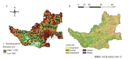
Fig.1 Sampling site distribution in Luanping County,Hebei Province,China.A,elevation map.B,land use map.

2.2.Collection and processing of soil samples

The sampling locations were determined using a stratified sampling method based on soil type,topography,and the spatial distribution of cultivated land in the county.A total of 789 topsoil samples (0-20 cm) containing the primary soil types in the study area were collected between 2016 and 2019 (Fig.1-A).For each sample,five different locations were randomly selected within a radius of 5 m of sampling sites,and the five subsamples collected from each sampling site were fully mixed into a composite sample.The geographical coordinates of each sampling site center were recorded using a portable global positioning system (GPS).The soil samples were air dried,stones and plant residues were removed,and the samples were then ground to pass through a 0.25-mm sieve.SOM was determined following the K2Cr2O7-H2SO4oxidation method (Nelson and Sommers 1996).

2.3.Synthesis of images and the construction of spectral predictors

Monthly image compositingA total of 566 Sentinel-2 images,Level-1C product (top of atmosphere (TOA) reflectance) with less than 10% cloud contamination,were chosen to cover the study area between January 1,2016 and December 31,2021.These images were radiometrically and geometrically corrected (Gattiet al.2015) and were archived on the GEE platform as the “Sentinel-2 MSI: multispectral instrument,level-1C” dataset.The median synthesis method,known for its efficiency and consistent results,was employed for optimal pixel selection (Luoet al.2022).The median value of spectral reflectance is less susceptible to potential extreme outliers than the mean value.Sentinel-2 images were synthesized in this study using the median indicators for each month over multiple years,and all composite images were resampled to a spatial resolution of 10 m.This process created 12 monthly synthetic images based on the Sentinel-2 data,and detailed synthetic information is shown in Table 1.

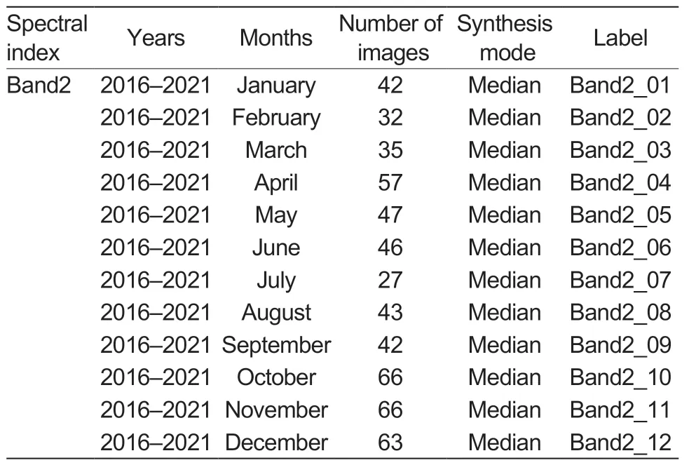
Table 1 Detailed synthetic information for Sentinal-2 imagery

Construction of monthly spectral indicesMonthly spectral indices were constructed using ten spectral bands including the blue band (Band2),green band (Band3),red band (Band4),and near-infrared band (Band8) which have a spatial resolution of 10 m,and the red edge band (Band5,Band6,Band7),near-infrared band (Band8A),and short-wave infrared band (Band11 and Band12) which have a 20 m spatial resolution.The three bands (Band1,Band9 and Band10) used for atmosphere correction have a spatial resolution of 60 m and were not utilized in this study.Three vegetation indices for each month were used to model the relationship with SOM (Penget al.2017).These indices include the normalized difference vegetation index (NDVI;Tucker 1979),the enhanced vegetation index (EVI;Hueteet al.2002) and the modified soil adjusted vegetation index (MSAVI;Qiet al.1994),and they were calculated as follows:

In summary,156 remote sensing variables were derived from the monthly synthetic Sentinel-2 images.

Combination of monthly synthetic spectral indicesAs a result of the limited spectral information contained in the synthetic images for a single month,multiple monthly composite images were grouped to explore the impact of different combinations of monthly synthetic variables on the accuracy of SOM mapping.Each set consisted of three consecutive months,corresponding to four quarters: Q1 (January to March),Q2 (April to June),Q3 (July to September) and Q4 (October to December).A total of 13 datasets were created by combining variables from single,two and three quarters within a year.These combinations were labeled Q1...Q12...Q234,and they were compared with the whole year (Q1234) in terms of their ability to predict SOM distribution.The overall flowchart was displayed in Fig.2.

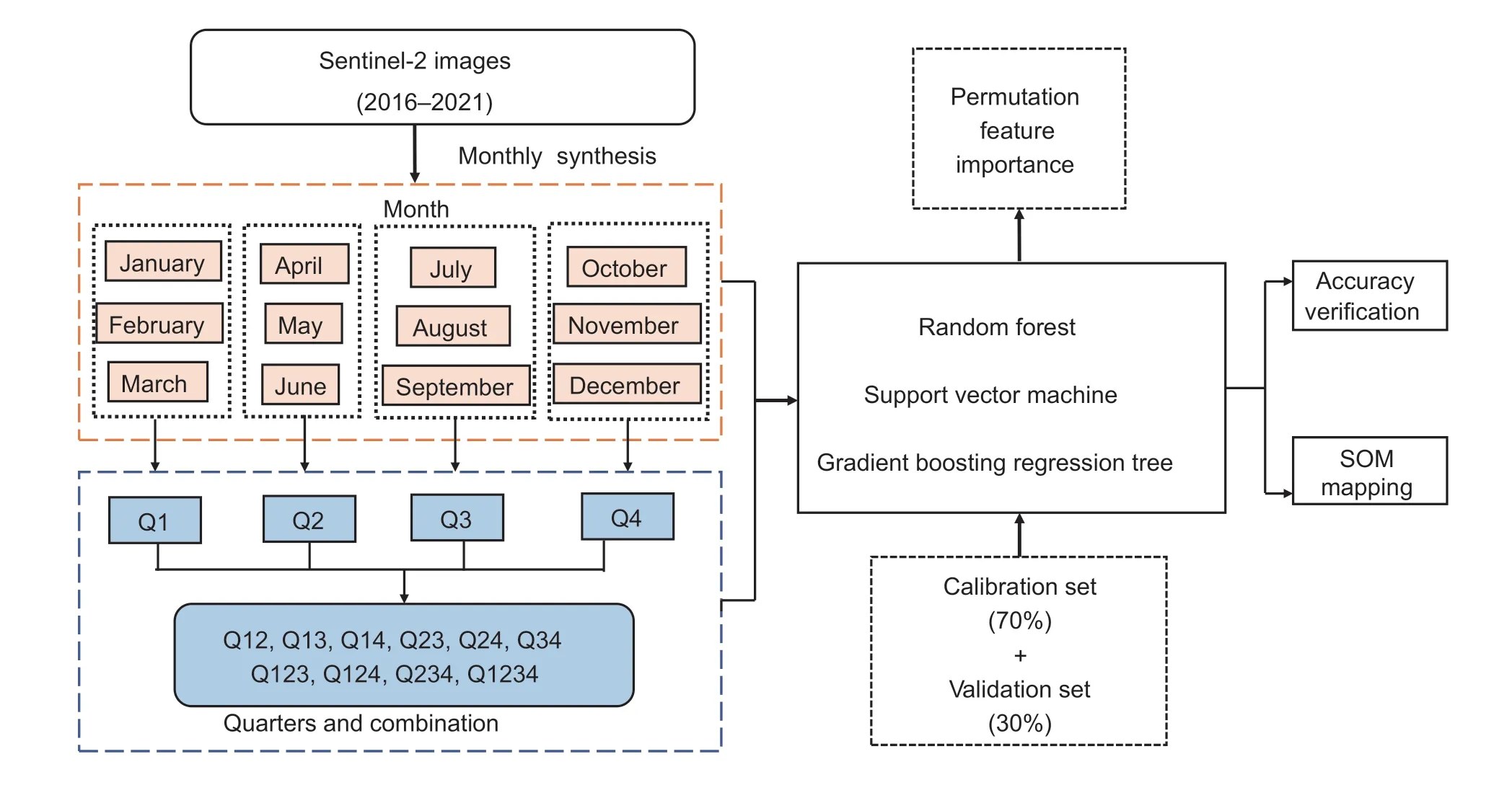
Fig.2 Flowchart of extracting spectral predictors using monthly synthetic images and their combinations for soil organic matter (SOM) mapping.

2.4.Modelling of soil organic matter

Random forest (RF)The RF algorithm,which integrates multiple trees through ensemble learning,was originally proposed by Breiman (2001).The Bootstrap sampling technique is applied to randomly selected samples from the training dataset to construct individual tree models and generate a number of trees to finally form the RF algorithm (Khanalet al.2018).The RF model is known for its resistance to overfitting and ability to generate stable and accurate predictions,which has led to its application in soil property mapping (Geet al.2022).

The RF model was implemented using the “randomForest” package in R 4.1.1 (R Development Core Team 2021).Two crucial parameters in the RF model that affect the accuracy of spatial prediction are the number of input features (mtry) at each splitting node and the number of decision trees (ntree).The optimal values for these parameters were selected using the grid search method from the “caret” package.

Support vector machine (SVM)SVM is a widely used supervised learning algorithm based on statistical learning theory (Cortes and Vapnik 1995).It is particularly suitable for handling high-dimensional feature data and has a low risk of overfitting (Padarianet al.2020;Ndepeteet al.2022).The SVM algorithm projects the data into a high-dimensional feature space by means of kernel functions.In the new space,the SVM seeks to find a hyperplane that can separate categories and create the widest margin between these categories (Forkuoret al.2017).The radial bias function (RBF) kernel function was selected for use in this study due to its demonstrated high performance in soil property prediction (Keskinet al.2019).

The “kernlab” package was utilized to develop the SVM model (R Development Core Team 2021).In the SVM modelling process,the optimization of gamma and cost (C) was achieved by the grid search method from the “caret” package.

Gradient boosting regression tree (GBRT)GBRT is a well performed ensemble learning approach,and it combines multiple decision trees based on stochastic gradient boosting techniques (Friedman 2001).A new regression tree in each iteration is constructed to optimize the loss function in the direction of the gradient of residual value reduction.This iterative process helps to reduce overfitting and enhance the robustness of the model (Chenet al.2019).

The GBRT model was implemented using the “gbm” package in R 4.1.1 (R Development Core Team 2021).Two important parameters in the GBRT algorithm are the number of iterations (n_estimators) and the learning rate.These parameters were tuned using the grid search method from the “caret” package.

2.5.Permutation feature importance (PFl) and partial dependence plots (PDP)

The importance of covariates in this study was assessed using the PFI method,which was first introduced by Breiman (2001) and further developed by Fisheret al.(2019).The strength of the PFI method is that it can be applied to any ML model.Given that SOM is a continuous variable,the importance of covariates was calculated based on the decrease in mean square error (MSE).A large reduction in MSE indicates a greater influence of the covariates on the target variable,as the model heavily relies on these variables for accurate predictions.The “iml” package in R 4.1.1 was used to analyze the importance of the 156 remote sensing variables in this study using the PFI method (Molnar 2018).

In order to understand the nonlinear relationship between the covariates and the target variable in the ML models,PDP was employed.PDP allows for visualizing the relationship between the target variable (SOM) and each input variable while holding all other variables constant.This enables the examination of the effect of individual variables on the prediction process.The “pdp” package in R 4.1.1 generated these plots and provided insights into the relationship between SOM and the input variables.

2.6.Accuracy verification

To evaluate the performance of the models,the 789 samples were randomly divided into two sets in the ratio of 7:3,with 546 training samples and 243 verification samples.The mean absolute error (MAE),root mean square error (RMSE) and coefficient of determination (R2) were used as metrics to assess the goodness of fit for the different models.Smaller RMSE and MAE values,and a largerR2value indicate better fitting performance.The computation of these metrics was as follows:

wherePiandOiare the predicted and observed SOM concentration at sitei,is the mean of all observed SOM values,andnis the number of soil samples.

3.Results

3.1.Descriptive statistics of SOM

The basic statistics for SOM concentration for the whole,calibration,and validation datasets are given in Table 2.The SOM concentration for the entire sample set ranged from 5.20 to 39.13 g kg-1,with a mean of 20.84 g kg-1and a standard deviation of 5.31.The coefficient of variation of the SOM concentration was 0.25,suggesting a moderate variability for SOM spatial distribution (Chaiet al.2021).The calibration and validation datasets had similar mean and standard deviation values to the entire dataset,indicating that they were representative subsets of the entire dataset.

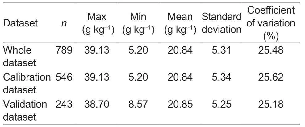
Table 2 Basic statistical analysis of soil organic matter in the study region

3.2.Correlations between monthly spectral variables and SOM concentration

A total of 156 spectral variables,including 120 spectral bands and 36 vegetation indices,extracted from the 12monthly-composited images,were utilized to predict SOM through three ML methods.The correlation analysis between the spectral data and SOM is presented in Table 3.When considering all months,the spectral reflectance of Band11 and Band12 exhibited the strongest correlations with SOM,followed by Band4 and Band5.Moreover,Band11 derived from all singlemonth composite images significantly correlated with SOM (P＜0.05).Among the calculated vegetation indices,NDVI and MASVI derived from composite images of April,May,June and October showed significant correlations with SOM.Furthermore,the spectral reflectance of all Sentinel-2 bands demonstrated significant associations with SOM (P＜0.05) in March,April,October,and November.

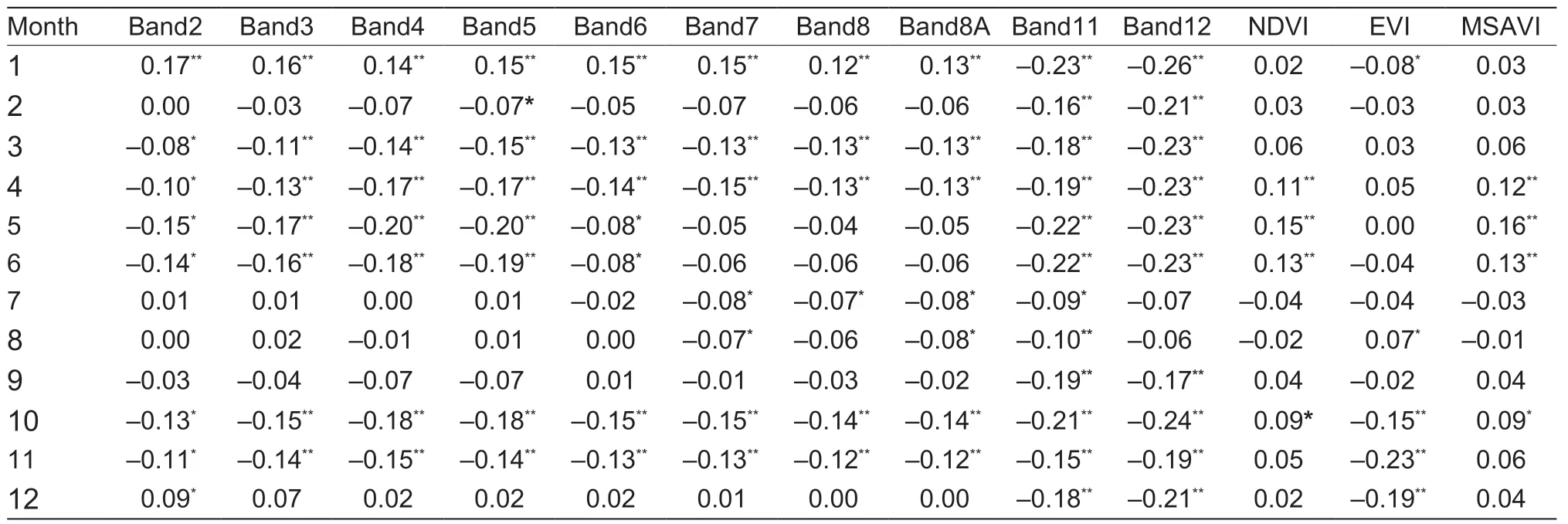
Table 3 Pearson’s correlation coefficients between soil organic matter and single-monthly synthetic spectral predictors1)

3.3.Assessing the predictive performance of all variable datasets

Comparison of prediction accuracy using singlemonth composite imagesFig.3 illustrates the performance of three modeling approaches (RF,SVM,and GBRT) across different months using the monthly synthesized images.TheR2value of all models exhibitedfluctuations corresponding to the timing of the synthetic images.For example,theR2value of the RF model decreased from 0.36 in January to 0.06 in July and then increased to 0.35 in December.Similar patterns were observed in the SVM and GBDT models.This fluctuation is also evident in the MAE and RMSE metrics.Notably,the synthetic images from November to March consistently demonstrated higher predictive performance than those from April to October.Furthermore,the RF model outperformed the SVM and GBRT models regarding estimation ability,as indicated by higherR2values and smaller MAE and RMSE.

Fig.3 Performance of three models for predicting soil organic matter in different months based on multi-year composite images.MAE,mean absolute error;RMSE,root mean square error;R2,coefficient of determination;GBRT,gradient boosting regression tree;RF,random forest;SVM,support vector machines.

Comparison of prediction accuracy for single-quarter and multiple quarter combinationsThe accuracy using variables from single-month synthetic images was low,suggesting that more spectral information was needed.The accuracy of different quarterly combinations and models was compared,and a summary of the results is given in Fig.4.In general,variables derived from multiple quarters achieved higher accuracy in predicting SOM than variables from a single quarter.

Fig.4 Performance of three models for prediction of soil organic matter under different combinations of quarters.MAE,mean absolute error;RMSE,root mean square error;R2,coefficient of determination;GBRT,gradient boosting regression tree;RF,random forest;SVM,support vector machines.

In terms of the single quarters,Q1 and Q4 exhibited higher accuracy than Q2 and Q3.Regarding twoquarter combinations,variables from Q14 achieved the highest accuracy in both the RF and SVM models (R2=0.50vs.R2=0.46,respectively),while variables from Q24 performed best in the GBRT model with anR2of 0.41.The prediction accuracies were similar across different combinations and ML models when considering three-quarter combination.As we expected,the highest prediction accuracy was obtained when variables from all quarters were utilized,and this data were used to generate scatter plots for the validation dataset (Fig.5).The evaluation metrics for SOM prediction models indicated that the RF model outperformed the SVM and GBRT models with anR2of 0.56,RMSE of 3.61 and MAE of 2.86.In comparison,the SVM model achieved anR2of 0.51,RMSE of 3.71,and MAE of 2.94,while the GBRT model yielded anR2of 0.44,RMSE of 4.01,and MAE of 3.20.Overall,the accuracy of the SOM prediction model improved as more variables from other months were included (Fig.4).However,the accuracy based on variables from Q23 was lower than that based on variables from a single quarter.This discrepancy could be attributed to the inability of all spectral variables from Q23 to effectively capture variation in SOM due to the influence of surface crop cover,soil moisture,etc.

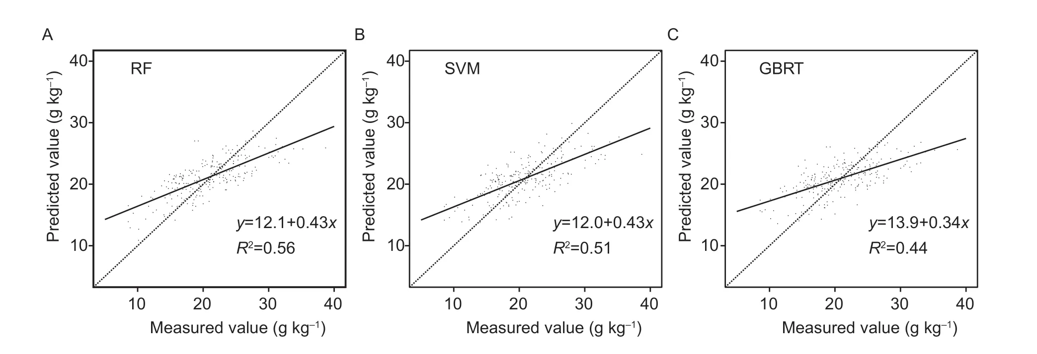
Fig.5 Comparison of scatter plots for the predicted and measured soil organic matter based on three models.A,random forest (RF).B,support vector machines (SVM).C,gradient boosting regression tree (GBRT).

In addition,the RF model consistently performed better than the SVM and GBRT models in predicting SOM concentration regardless of the variables incorporated in the models.

3.4.lmportance of environmental variables and partial dependence plots

The permutation feature importance (PFI) (%),as shown in Fig.6,revealed the significance of the top 30 covariates in the RF,SVM,and GBRT models.It was evident that Band12_12 strongly impacted the prediction of SOM in all three models.The remaining variables showed relatively similar permutation feature importance scores.Among the vegetation indices,EVI_11 and EVI_04 were ranked higher in importance,while NDVI and MSAVI had less influence on predicting SOM.In addition,when considering the 30 covariates,approximately 40,50,33%,and 27,23,23% of the variables derived from Q1 and Q4,were identified as important by the RF,SVM,and GBRT models,respectively.This implies that the monthly synthetic variables from Q1 and Q4 exhibit higher SOM prediction accuracy than other quarters.

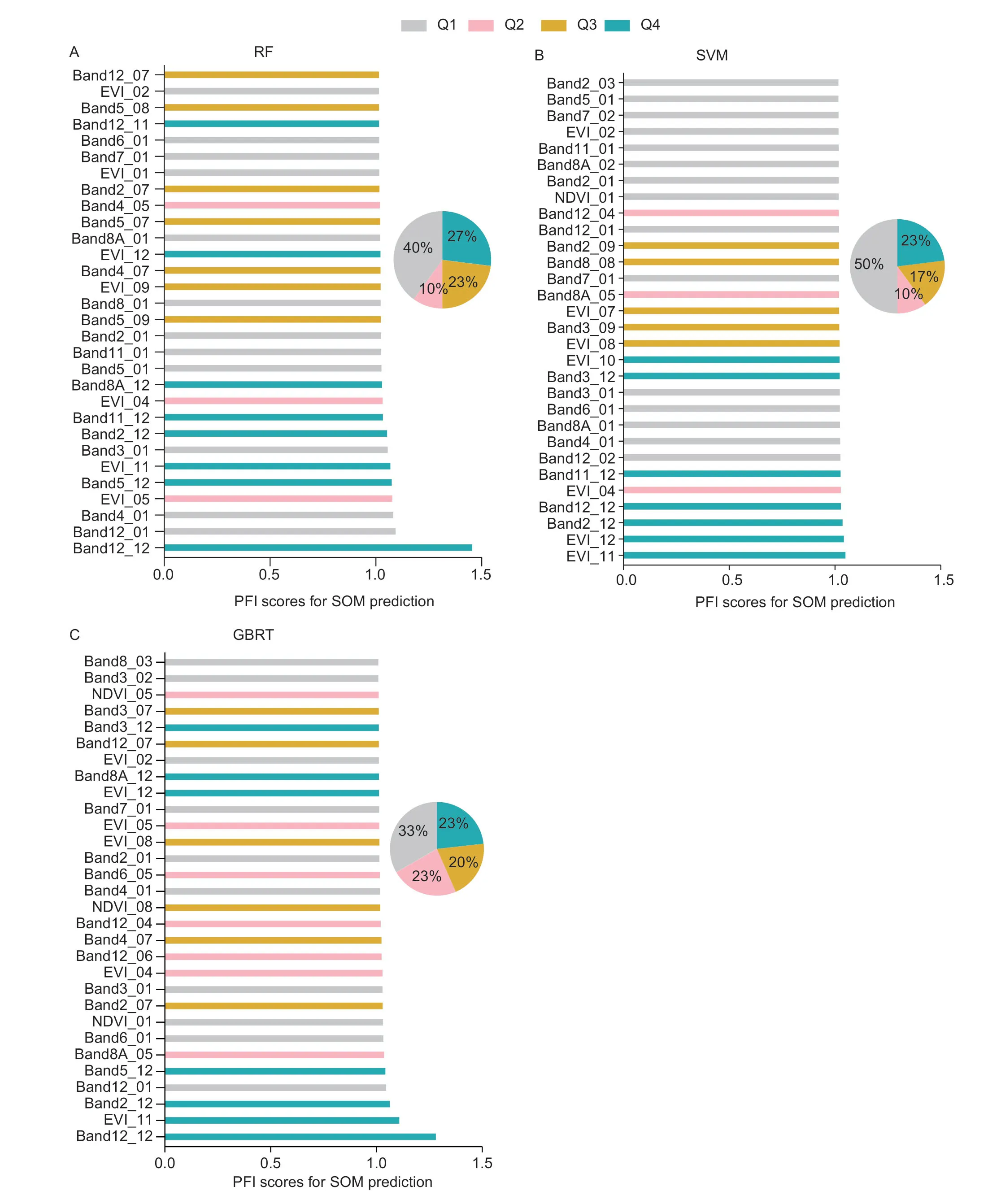
Fig.6 A comparison of the relative importance ranking of the top 30 covariates in soil organic matter (SOM) prediction using different models for predicting SOM.A,random forest (RF).B,support vector machines (SVM).C,gradient boosting regression tree (GBRT).PFI,permutation feature importance.

PDP were generated for the top three influential covariates and are displayed in Fig.7.These plots illustrate how the SOM concentration tends to change as a function for each covariate.The PDP results revealed diverse shapes of fitted functions and obvious non-linear relationships,particularly in the RF and GBRT models.In these models,regions with high SOM concentration associated with Band12_12 values ranging from 1,000 to 2,000,whereas the SOM concentration sharply decreased when band values exceeded 2,000.Similar trends were observed with the Band12_01 in the RF model.Additionally,in the SVM model,the gradually decreasing SOM concentration was linked to a slow increase in EVI_11 and EVI_12 values,demonstrating the capability of vegetation indices to capture soil variability.

Fig.7 Partial Dependence Plots (PDPs) of the top three influential covariates for predicting soil organic matter based on three models.A,random forest (RF).B,support vector machines (SVM).C,gradient boosting regression tree (GBRT).

3.5.Spatial characteristics of SOM maps

The spatial distribution of organic matter in cultivated soils based on the RF,SVM,and GBRT models,utilizing all monthly synthetic variables,are illustrated in Fig.8.The maps generated by these prediction methods exhibit a similar overall pattern,displaying a discontinuous distribution of SOM at the regional scale.Areas with higher elevations,particularly in the northeast and southeast regions,tend to have higher SOM values,indicating the accumulation of SOM resulting from limited human activities.Conversely,lower SOM values are predominantly observed in the river valley area,characterized by relatively low terrain and greater human activity.However,noticeable differences in spatial patterns are evident between the maps generated by the RF model and those produced by the GBRT and SVM models.The maps generated by the RF model exhibit smoother transitions between boundaries than the SVM and GBRT models.Furthermore,the RF algorithm produced SOM concentrations ranging from 8 to 36 g kg-1,which aligns more closely with the measured values than the SVM (10 to 32 g kg-1) and GBRT (10 to 31 g kg-1) models.

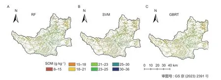
Fig.8 Soil organic matter (SOM) map with a resolution of 10 m based on three models.A,random forest (RF).B,support vector machines (SVM).C,gradient boosting regression tree (GBRT).

4.Discussion

4.1.Variation in monthly synthetic spectral information

The observed variation in the correlations between SOM concentration and Sentinel-2 spectral variables for many months can be attributed to the changing soil moisture content and surface vegetation conditions over time.The study by Guoet al.(2021) supports this notion by demonstrating that vegetation growth variation can influence the relationships between spectral information and soil properties.Similarly,Minhoniet al.(2021) emphasized the correlation between spectral indices and organic carbon was significant in June,July,and August,during the dry winter period in Brazil.Therefore,the influence of temporal variation in spectral indices over the year on SOM mapping should be assessed.

The significant correlations observed between SOM and the spectral reflectance of two short-wave infrared (SWIR) bands,Band12 and Band11,for almost all months indicate the importance of these bands in SOM modeling.The variable importance analysis further highlighted the significance of Band12 in December for SOM prediction.This can be attributed to the fact that the main components of organic matter,such as cellulose,lignin and starch,can influence the spectral reflectance around 2,100 and 2,300 nm (Ben-Doret al.1997).Castaldiet al.(2019) also demonstrated that although the spectral bands in the SWIR region are relatively broad,they are effective in capturing the correlation between SOM concentration and the spectral signature reflected by SOM in the study area.The significant correlations between SOM and the reflectance values in the visible (VIS) bands (Band2,Band3,Band4) for most months can be attributed to the presence of typical absorption features of SOM within the VIS spectra (Viscarra Rosselet al.2011).Moreover,Changet al.(2001) revealed an inverse relationship between SOM concentration and the albedo of the visible near-infrared (VNIR) band,highlighting the importance of VNIR bands in SOM prediction.However,it is worth noting that,in this study,except for B7,the VNIR bands (Band5,Band6,Band7,Band8,Band8A) exhibited a weak correlation with SOM in July,August,and September.This could be attributed to lush surface vegetation during the summer,which might have influenced the availability of soil spectral reflectance in those specific bands (Wanget al.2020).

Based on PFI analysis,EVI played a more important role in predicting SOM than NDVI and MSAVI in most months.This is probably because EVI is more sensitive to changes occurring in crop canopies,enabling it to effectively mitigate the influence of cover crops on SOM prediction (Hamzehpouret al.2019).A negative correlation between SOM and EVI was observed during most months,which aligns with the findings of Minhoniet al.(2021).

4.2.Application of monthly synthetic spectral variables

The study demonstrates the potential of SOM prediction utilizing synthetic spectral variables every month.However,when employing variables obtained from singlemonthly composite images,the overall accuracy of the SOM prediction model is relatively low,withR2ranges from 0.06 to 0.36 for the RF model,0.04 to 0.31 for the SVM model,and 0.08 to 0.34 for the GBRT model.The results indicate that the spectral information in singlemonthly composite images may not adequately capture the spatial variation of SOM concentration.Additionally,the accuracy variation of SOM prediction using variables from a single month exhibited similar patterns throughout the year for all three models.Interestingly,the accuracy was higher in January and December compared to the other months,which can be attributed to the following two reasons.Firstly,corn is the primary agricultural crop in this region and is typically planted around mid-March and harvested around mid-September.As a result,the cultivated land experiences minimal crop coverage during winter,when there is a period of bare soil.Secondly,higher soil moisture levels tend to decrease soil reflectance,which may affect the characteristics of the spectral profile and the absorption features (Baumgardneret al.1986).Thus,the lower soil water content during winter can be advantageous for SOM mapping.

This study also demonstrated that utilizing variables from more monthly Sentinel-2 synthetic imagery could yield more reliable SOM predictions,which may be due to the fact that more monthly synthetic variables can provide more available information related to SOM.Thus,the SOM prediction model based on the full-year Sentinel-2 monthly-synthesized dataset gave the best results,with the lowest RMSE and MAE,and the highestR2.Similarly,Zhanget al.(2019) explored the influence of NDVI time series data of summer crop production on soil organic carbon in the Jianghan Plain of China,and found that using NDVI derived from a single month or a short time series resulted in lower estimation accuracy than using NDVI from long time series.Yang (2021) also showed that the accuracy of predicting SOM achieved obvious improvement when the dead fuel index (DFI) and NDVI from the four quarters were incorporated into the models.However,Zeraatpishehet al.(2022) performed a comparative analysis on the effectiveness of common topography covariates and combinations of vegetation indices derived from Sentinel 2 images at different months for SOC prediction,and the results showed that the accuracy did not show improvement when incorporating time-series vegetation indices.This condition was because the time series vegetation indices were extracted from single-year data rather than multi-year composite images,which was susceptible to atmospheric noise.

4.3.Performance of machine learning models

Differences in the accuracies of SOM prediction among the three ML algorithms were observed in this study.The RF model consistently outperformed the SVM and GBRT models in predicting SOM using various monthly synthetic variable datasets.This superior performance of the RF model can be attributed to its greater ability to reduce sensitivity to overfitting and to effectively handle nonlinear and hierarchical relationships between input predictors and the target soil properties (Akpaet al.2016).For instance,Kayaet al.(2022) compared three popular ML methods to estimate soil texture classes,and the results revealed that the RF model yielded the highest prediction accuracy.Fathizadet al.(2022) also showed that the RF model achieved a higher accuracy than the SVM model and artificial neural networks .Additionally,Mahmoudzadehet al.(2020) found that the RF model achieved the highest accuracy in predicting SOC in western Iran.

The GBRT model performed better than the SVM model when predicting SOM using single monthly images.However,when utilizing different quarterly images and their combinations,the SVM model outperformed the GBRT model.This discrepancy in performance may be attributed to the variation in the spectral information captured from the monthly synthetic images incorporated into the respective models.Indeed,the performance order of ML algorithms is not always consistent and can be influenced by geographic location,sampling density and design,and the selection of environmental variables (Zhouet al.2021).This is why different performance statistics for different ML algorithms have been reported in different studies (Munnaf and Mouazen 2022).

4.4.Limitations and prospects

Although our findings demonstrated improved accuracy in SOM prediction using variables obtained from multiyear synthetic Sentinel-2 images,there are still some limitations for improvement using spaceborne data.Common spaceborne platforms,such as multispectral and hyperspectral,as well as radar sensors offer images with different spectral,spatial and temporal resolutions.However,due to sensor technology constraints,there is a trade-off between these resolutions,making it challenging to achieve high resolution in all three aspects simultaneously (Dianet al.2021;Chenet al.2023).For example,when comparing multispectral sensors to hyperspectral data,the latter possesses a higher spectral resolution due to its hundreds of narrow bands.However,hyperspectral data has limited spatial and temporal coverages and is hard to be implemented for soil property prediction across large regions (Wanget al.2023).In addition,optical satellite imagery is susceptible to cloud cover,but synthetic aperture radar (SAR) offers the advantage of all-day and all-weather monitoring despite its relatively low resolution and low signal-to-noise ratio (Lauschet al.2016).Consequently,multi-source remote sensing data fusion can be considered to further improve the performance of SOM prediction.

Since spaceborne sensors are carried at hundreds of kilometers above the Earth,atmospheric interference,noise and distortion emerge as the main limiting factors for the interpretation of satellite images.Gelsleichteret al.(2023) found that incorporating multispectral bands from Sentinel-2 along with laboratory Vis-SWIR spectra could effectively enhance soil mapping because the soil laboratory Vis-SWIR spectra signals were free from atmospheric influence and vegetation cover.Additionally,surface relief can influence optical images in mountainous regions,leading to shadows and variations in reflectance levels.This can result in unwanted heterogeneity in surface imagery,potentially impacting the accuracy of soil mapping efforts.

5.Conclusion

This study presents a method for accurately predicting soil organic matter (SOM) concentration in cultivated soil using monthly synthetic Sentinel-2 MSI data.A total of 789 soil samples and Sentinel-2 monthly synthetic images acquired from 2016 to 2021 covering the study area were collected.The extracted band information and spectral indices were then employed to develop SOM prediction models using three machine learning algorithms: RF,SVM,and GBRT.Regarding the spectral index variables obtained from 12 single-month synthesized images,the models based on variables from January and September showed a better accuracy compared to the other months.It was found that Band12 in December played a crucial role in predicting SOM concentration.

The general accuracy of predicting SOM based on variables for a single-month was poor.However,as more monthly spectral indices were incorporated into models,the prediction accuracy of SOM improved.The highestR2value,along with the lowest mean absolute error (MAE) and root mean squared error (RMSE),were observed when the spectral variables from all months of the year were combined together.Moreover,the RF model achieved better prediction accuracy (MAE=2.86,RMSE=3.61 andR2=0.56) using monthly synthesized Sentinel-2 images than the SVM and GBRT models.The findings of this study provide a reference for mapping SOM using monthly synthetic Sentinal-2 images.

Acknowledgements

Funding and resources for this study came from the special project of the National Key Research and Development Program of China (2022YFB3903302 and 2021YFC1809104).

Declaration of competing interest

The authors declare that they have no conflict of interest.