Automatic modulation recognition of radiation source signals based on two-dimensional data matrix and improved residual neural network

Gunghu Yi , Xinhong Ho ,b, Xiopeng Yn ,b,*, Jin Di , Yngtin Liu ,Ynwen Hn

a Science and Technology on Electromechanical Dynamic Control Laboratory, School of Mechatronical Engineering, Beijing Institute of Technology, Beijing 100081, China

b BIT Tangshan Research Institute, Beijing 100081, China

Keywords:Automatic modulation recognition Radiation source signals Two-dimensional data matrix Residual neural network Depthwise convolution

ABSTRACT Automatic modulation recognition (AMR) of radiation source signals is a research focus in the field of cognitive radio.However, the AMR of radiation source signals at low SNRs still faces a great challenge.Therefore, the AMR method of radiation source signals based on two-dimensional data matrix and improved residual neural network is proposed in this paper.First,the time series of the radiation source signals are reconstructed into two-dimensional data matrix, which greatly simplifies the signal preprocessing process.Second, the depthwise convolution and large-size convolutional kernels based residual neural network (DLRNet) is proposed to improve the feature extraction capability of the AMR model.Finally, the model performs feature extraction and classification on the two-dimensional data matrix to obtain the recognition vector that represents the signal modulation type.Theoretical analysis and simulation results show that the AMR method based on two-dimensional data matrix and improved residual network can significantly improve the accuracy of the AMR method.The recognition accuracy of the proposed method maintains a high level greater than 90% even at -14 dB SNR.

1.Introduction

AMR is a technology that automatically recognizes the modulation type of unknown signals in the non-cooperative state [1].AMR is widely used in the fields of radiation source classification,information interception, jamming recognition, and spectrum awareness [2].However, with the development of signaltransmitting technology, signal modulation types have become diversified.Signals of different frequencies and different modulation types fill the electromagnetic space [3-5].The received radiation source signals from radio fuze and radar are filled with a lot of jamming and noise.Effective recognition of the modulation type of the radiation source signals at low SNR is a hot topic of current research.Therefore, many scholars have conducted numerous studies on this subject [6-8].

Signal modulation and modulation-type recognition are dynamic game processes.AMR technology tends to evolve along with signal modulation technology.In the early development of AMR technology,scholars have proposed many effective schemes based on traditional signal processing methods.Some methods that use pulse descriptors as feature parameters [9,10] are effective in scenarios with fewer signals and simpler modulation forms.However,as the type of signal modulation becomes more complex, the performance of these methods decreases.To deal with complex forms of signals, scholars have proposed more distinguishing features.Wang et al.[11] proposed a modulated signal recognition method based on the signal spectrum and instantaneous autocorrelation.The method distinguishes phase-modulated signals from FM signals based on the amplitude and phase characteristics of the instantaneous autocorrelation signals.Zhang et al.[12]proposed a method based on the fractional-order Fourier transform and circular spectrum for signal modulation-type recognition.Hussain et al.[13] proposed a feature extractor based on higher-order accumulation and a genetic algorithm for signal feature extraction,and the k-nearest neighbor algorithm was used to classify the five modulated signals.Liu et al.[14]proposed a method based on scale-invariant feature transform (SIFT) to extract signal features and then perform feature classification by support vector machine(SVM),which achieved good recognition results.

The above methods have achieved good results in AMR tasks.However,artificial signal feature extraction relies on strong a priori knowledge, and the recognition process is tedious and computationally complex.Due to the rapid development in the field of deep learning (DL), many scholars have applied the achievements of DL to AMR tasks.DL models have strong feature extraction capability and can extract data features autonomously for learning.

Yu et al.[15] extracted the normalized signal time-frequency image by short-time Fourier transform (STFT), then used a noise reduction network for noise reduction.Finally, the noise-reduced time-frequency images were recognized by the residual neural network.When the SNR was higher than -10 dB, the recognition accuracy reached 90%.The signal time-frequency image extracted by STFT and classified by the CNN is also available in Refs.[16-18].Li et al.[19]used the Wigner-Ville distribution to extract the timefrequency image of the signal and used the DL model for classification.When the SNR was higher than -5 dB, the recognition accuracy reached 75%.The literature [20,21] extracted the signal time-frequency image by smoothed pseudo-Wigner-Ville distribution and inputting the time-frequency image into the CNN to recognize the modulation type of the signal.The above AMR method has achieved good results by using DL models for signal feature extraction, which has improved the autonomy of AMR technology to a certain extent.However, using time-frequency analysis for signal preprocessing still relies on strong a priori knowledge.In the time-frequency analysis process,signal window function selection relies on professional experience and much experimentation.The effect of time-frequency analysis is directly influenced by the number of data points, the window function length, or the wavelet basis type.Therefore, in previous studies,scholars have mostly used desirable time-frequency images as the input of DL models for recognition.

To further eliminate the dependence on a priori knowledge and increase the autonomy of AMR methods, in this paper, signal preprocessing is simplified by directly processing the time-domain signals intercepted by radar receivers.Before the method proposed in this paper, AMR methods that directly deal with timedomain signals were also proposed.Wang et al.[22] input the IQ time-domain signals of multiple radiation source signals into a DL model for modulation-type recognition.When the SNR is above-5dB, the recognition accuracy is higher than 65%.Zou et al.[23]used a DL model with a self-attentive mechanism and a long shortterm memory(LSTM)mechanism to recognize the modulation type of IQ time-domain signals and achieved a recognition rate of 70%above -5 dB.In the literature [24-27], IQ time-domain signals of the radiation source signals are used as inputs to the model for the AMR task.

In the above method, the time series of the radiation source signals are used as model input, which improves the autonomy of the AMR method.However, the length of the input onedimensional sequence is limited by the processing performance of current DL models.For signals with large modulation periods,the limited data length cannot fully characterize the modulation characteristics of the signal, which can lead to lower recognition rates.When the length of the input sequence is large, the time series model needs to have memory capability or global feature extraction capability as a method to obtain the global features of the signal,which will increase the model complexity and consume more computational resources.

In this paper,the AMR method of radiation source signals based on two-dimensional data matrix and improved residual neural network is proposed to improve the degree of autonomy of AMR methods and expand the application scenarios.

First,a signal preprocessing method based on two-dimensional data matrix for AMR is proposed.Compared with time-frequency images and IQ data, the two-dimensional data matrix can not only reduce the dependence on a priori knowledge and improve the autonomy of signal preprocessing in the AMR process but also take advantage of matrix computing to increase the length of the input signal sequence and reduce the computational cost.

Second,the network structure of the residual neural network is improved for the input of the two-dimensional data matrix in the recognition process.The depthwise convolution and large-size convolutional kernels based residual neural network (DLRNet) is proposed for processing two-dimensional data matrix based on time series reconstruction.The DLRNet model can effectively improve the accuracy of AMR methods at low SNR.

Finally, compared to the current advanced AMR technology.Simulation results show that the AMR method based on twodimensional data matrix and improved residual neural network can significantly improve the recognition performance of the AMR method.The recognition accuracy of the proposed method maintains a high level greater than 90% even at -14 dB SNR.

2.AMR method of radiation source signals

The AMR method of radiation source signals based on twodimensional data matrix and improved residual network is divided into the following steps.First, the signals of radiation sources with different modulation types in the electromagnetic space are acquired by radar receivers.A mixer mixes the intercepted signal to obtain the IF signal.The time series of the IF signal is then converted into a two-dimensional data matrix according to specific processing.Then, a radiation source signals modulationtype recognition model is established, which is trained by learning the radiation source signals dataset features.Finally, the model recognizes the two-dimensional data matrix of the acquired radiation source signals and outputs a one-dimensional recognition vector indicating the radiation source signals modulation type.

2.1.Recognition process

Assume that the type of signal modulation type is N.The output vector Y of the model is a one-dimensional matrix of length N.The elements of this one-dimensional vector all consist of 0 and 1.The radiation source signals of different modulation types are one-heat encoded in a specific order.For example,when the modulation type of the radiation source signals is pulse modulation,the vector Y has a value only when the subscript n =3,and the rest of the values are 0.

The radiation source signals are preprocessed to obtain a twodimensional data matrix.The two-dimensional data matrix is used as the input to the AMR model.In Fig.1, the function fDLRNetmaps the two-dimensional data matrix to obtain a onedimensional recognition vector.

2.2.Signal preprocessing method

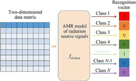
Fig.1.The recognition process of the AMR model.

The one-dimensional time series are transformed into a twodimensional data matrix using sequential alignment.This approach preserves the complete relationship of signal amplitude with time and transforms it into a relationship of signal amplitude with position.In CNNs, a common inductive bias is that features have local correlation.For time-domain signals, the correlation between neighboring amplitude points is greater than that between points that are farther apart.The signal preprocessing method for reconstructing a two-dimensional data matrix by time series enables the combination of the local signal correlation with the inductive bias of the CNN, which facilitates the model to learn the essential signal features.

The segment extraction process of a one-dimensional time series is adopted in the form of data slicing.One-dimensional time series data of different lengths are extracted according to different application scenarios.The extracted data are arranged chronologically as a two-dimensional data matrix with length and width L.The process is shown in Fig.2.

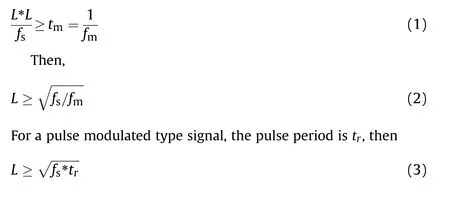
A two-dimensional data matrix contains a segment of the time series signal of length L*L.When L =60,the time series signal has LS=3,600 data points; when L = 180, the time series signal has LS=32,400 data points;and when L =240,the time series signal has LS=57,600 data points.As L increases, the number of data points increases in multiples of the square,and more signal features are contained in the two-dimensional data matrix.When a suitable size L is selected,the two-dimensional data matrix contains enough signal features for the DL model to learn the data features.

When data interception is performed on the signal time series,the length of the intercepted time series contains at least one full signal modulation period.When there are signals of multiple modulation types, the minimum value of the intercepted time series length must be greater than the maximum modulation period of the signals of different modulation types.

Assume that the center frequency of the signal is fb.According to Nyquist’s sampling theorem,the sampling frequency of the signal is fs≥fb.In practice, more than 5 equal to the center frequency is selected as the sampling frequency, which is fs≥5fb.The modulation frequency of the FM signal is fm, and the corresponding modulation period is tm= 1/fm.With a sampling frequency of fs,

2.3.Two-dimensional data matrix of the radiation source signals

In computer storage, image data are also a two-dimensional matrix.The color image consists of a two-dimensional matrix with three channels, and the grayscale image consists of a twodimensional matrix with a single channel.Whether a general image or a time-frequency image, the image pixel points are highly correlated, and there is a certain variation gradient in the pixel points in adjacent regions.The correlation and pixel change gradients reflect the image content and features.The convolution calculation of an image will extract features using the correlation between pixel regions.

The value of each point of the two-dimensional data matrix based on the time series reconstruction represents the signal amplitude.Since the input radiation source signals is at a low SNR,the signal carries a large amount of noise and jamming signals.At low SNRs, the amplitude variation in the signal is more random,and the amplitude points show a random distribution in the twodimensional matrix.The correlation between amplitude points is also greatly reduced,and the gradient changes in adjacent regions are more random.Therefore,it will become more difficult to extract the features of the signal by convolution calculation.

In Figs.3 and 4,the characteristics of the two-dimensional data matrix based on time series reconstruction are shown in the form of three-dimensional stereo images as well as two-dimensional flat images.As shown in the Figure, the location of the pulse is easily distinguished at a high SNR.As the SNR gradually decreases and the useful signal is drowned in the noise, the data distribution of the two-dimensional matrix shows a random distribution.The correlation between adjacent amplitude points is reduced, and the gradient changes are promiscuous.

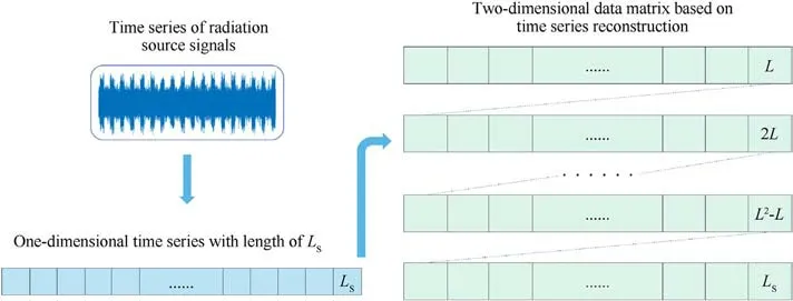
Fig.2.The process of transforming the radiation source signals into a two-dimensional data matrix.

Fig.3.Three-dimensional plot of the LFM pulse compression signal.L = 180: (a) SNR = 5 dB; (b) SNR = 0 dB; (c) SNR = -5 dB.

Fig.4.Two-dimensional image of the LFM pulse compression signal.L = 180: (a) SNR = 5 dB; (b) SNR = 0 dB; (c) SNR = -5 dB.

Based on the above analysis, the complexity of the twodimensional data matrix based on time series reconstruction is much higher than that of data such as time-frequency images.To adapt to the input of a two-dimensional data matrix, this paper proposes an improved residual neural network based on depthwise convolution and a large convolution kernel for feature extraction and radiation source signals recognition.

3.Recognition model construction

For the two-dimensional data matrix characteristics, an improved residual neural network model based on depthwise convolution and a large-scale convolution kernel is proposed in this paper.The DLRNet uses a depthwise conv layer with a large convolutional kernel as the basic convolutional computational unit.Depthwise convolution is used to extend the network width and reduce the model complexity.Large convolution kernels are used to increase the model perceptual field and improve the feature extraction capability.

DLRNet consists of a feature extraction module and a classification module cascade.The feature extraction module consists of five mixed depthwise convolution blocks(MDCBs).A convolutional block (CB) and two depthwise convolution residual blocks (DRB)are included in the MDCB.The classification module consists of a cascaded flatten layer, a dense layer, an activation layer, and a dropout layer.The network structure and data processing flow of DLRNet are shown in Fig.5.

3.1.Convolution block

The CB consists of a 1 × 1 conv layer and a linear activation function layer.The 1 × 1 conv layer traverses each element of the input two-dimensional data matrix and expands the number of input data channels.The linear activation function mapping relation is a constant transformation that does not change the input and acts as a network connection.Although the 1 × 1 conv layer consumes considerable computational resources, it can effectively extract the nonlinear features of the two-dimensional matrix during data traversal,which serves as an information fusion function,which helps to improve the feature extraction ability of the model.

3.2.Depthwise convolution residual block

The DRB is a key part of the DLRNet model.The DRB uses a depthwise conv layer of size 9 × 9 with a sliding step of 1.Depthwise convolution is a grouped convolution type where a single convolution filter is applied to each input channel.Depthwise convolution belongs to grouped convolution.In the depthwise convolution computation, the input is first split into individual channels, and then the depth kernel is used to perform the convolution operation with each input.Finally, the outputs of the convolution are superimposed along the channel axes.Unlike regular convolution, depthwise convolution does not mix information between input channels.The calculation results of each channel are fed into the next layer independently and in parallel with each other.The independent convolution computation of depthwise convolution does not need to calculate the fusion results of each channel,which can greatly reduce the computational effort.In both ResNeXt[28]and ConvNeXt[29],group convolution is used to widen the network width and reduce the network complexity.

During the convolutional computation, the size of the convolutional kernel determines the size of the perceptual field.For any element of a layer, its perceptual field is all the elements that affect the calculation of that element during forward propagation.The larger the size of the convolution kernel is, the larger the perceptual field.The large size of the convolution kernel enables better signal depth feature extraction.However, the convolution kernel is not as large as possible.As the convolution kernel becomes larger, the model becomes more computationally intensive.When the convolutional kernel reaches a certain size, the performance gain from continuing to increase the size is small,but the computational gain is large.The gold standard for convolution kernels starting from VGGNet [30] is 3.With the development of DL, there are also scholars who use larger convolution kernels for computation.Good results were achieved in ConvNeXt[29]using a 7 × 7 conv layer.

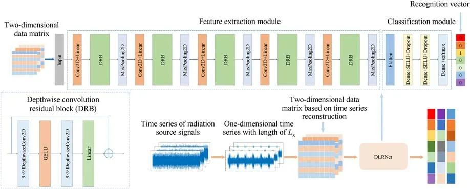
Fig.5.AMR model based on two-dimensional data matrix and improved residual neural network.

The initial convolution kernel size of the model is 3.However,the model performance improvement effect brought by changing other structures is insufficient to meet the recognition accuracy requirement.Therefore, the size of the convolution kernel is improved to obtain better feature extraction capability for the input data characteristics.The recognition effects of convolutional kernels of sizes 3, 5, 7, 9, and 11 were tested experimentally.The experimental results show that the 9×9 convolution kernel is the most effective for model enhancement.

In the DRB,the first depthwise conv layer is connected after the GELU activation function layer, and the second depthwise conv layer is connected after the linear activation function layer.The Gaussian error linear unit (GELU) [31] is a smooth rectified linear unit (ReLU) variant.It is currently used in advanced models,including Google’s BERT [32] OpenAI’s GPT-2 [33], and ConvNeXt[29].The GELU activation function is also applied in DLRNet to improve the model performance.The approximate expression of the GELU activation function is shown in Eq.(4).

3.3.Mixed depthwise convolution block

The MDCB is the main component of the DLRNet feature extraction module.The feature extraction module consists of an input layer and five MDCBs.The MDCB consists of a CB, two DRB and a max pooling layer cascade.

Depthwise convolution does not mix the convolution results of each channel.CB is added to the beginning of each MDCB to avoid using depthwise convolution, destroying the correlation between the data of each channel and losing regionally relevant features.The 1×1 conv layer can both traverse the two-dimensional matrix data to extract the nonlinear data features and fuse the channel data with the depthwise convolution results in the previous MDCB layer to extract the joint features between channels and improve the model performance.

A pooling size of 2 × 2 is used for the max pooling layer.The feature maps are dimensionally reduced by pooling calculation.After each pooling calculation,the size of the feature map is halved,and the number of channels remains the same.The max pooling layer enhances the discrimination between features, strengthens the scale invariance of image features and alleviates the oversensitivity of the convolutional layer to position.

3.4.Classification module

After the feature extraction module completes the feature extraction for the input data, the multichannel feature map is obtained.The feature map is transformed into a single-channel onedimensional feature vector in the flatten layer.The length of the feature vector is then further compressed by the dense layer to improve the distinguishability of the features.

A nonlinear activation function layer is added after the dense layer to prevent the model from degenerating into a linear model due to full connectivity.The nonlinear activation function used after the dense layer is the scaled exponential linear unit (SELU)[34].SELU is a variant of ReLU.The expression of the SELU activation function is shown in Eq.(5).

After passing through the SELU activation function layer, the data enter the dropout layer.The dropout method is a common method for training neural networks, which achieves the effect of artificially adding noise by discarding some of the neuron nodes.The dropout method effectively improves the generalization ability of the model and reduces the overfitting phenomenon during model training.In the classification module of DLRNet, the dense + SELU + dropout structure is used twice.The numbers of neurons in the dense layer are 128 and 64.The dropout probability is 0.5.

The final DLRNet output layer consists of dense layer and activation function layers.The number of neurons in the dense layer is the total number of radiating source signal modulation types.The dense layer can finally converge the model output to the total number of categories to be classified and output a one-dimensional vector of length N.This one-dimensional vector contains the probabilities for each modulation type.Finally, the softmax activation function maximizes the probability of the observed data.The softmax function transforms an unnormalized prediction into a nonnegative number and sums to 1.

After the softmax activation function layer,the model outputs a one-dimensional recognition vector of length N, consisting of values 0 and 1 to represent the corresponding radiation source signals modulation type.

3.5.Loss function

The loss function is used as an evaluation tool to quantify the difference between the actual and predicted target values,and the type of loss function directly affects the effectiveness of the model fit.The DLRNet input data are labeled with one-hot encoding.The prediction labels output by the model are one-dimensional vectors consisting of 0 and 1.According to the input and output characteristics,the loss function used by DLRNet is the categorical crossentropy loss function.The cross-entropy loss function describes the similarity between the actual and desired output probability.The smaller the cross-entropy value is, the closer the two probability distributions.The categorical cross-entropy loss function is used to calculate the cross-entropy loss between labels and predictions and is mostly used in label-oriented multiclassification problems.

3.6.Optimization algorithm

During the training process,the optimization algorithm is used to optimize the value of the loss function.The gap between the predicted and true values is reduced by continuously decreasing the value of the loss function to indirectly optimize the model.Since the radiation source signals is at a low SNR level, the useful signal is drowned in the noise.The input data exhibit random distribution characteristics.As a result,there are a large number of saddle points in the model optimization process, which leads to lower model convergence efficiency.

The stochastic gradient descent method with momentum(SGDM) and the Adam adaptive optimization algorithm are compared in the model training process.The mainstream Adam algorithm has good adaptive performance and enables the model to converge quickly to a better performance point.However, the model appears to be overfitted and oscillates repeatedly within the saddle point and cannot effectively escape the saddle point to achieve better accuracy.Compared with the Adam optimization algorithm,which has good adaptive performance,SGDM performs better in the face of low SNR signals with more random data distribution and enables the model to reach higher accuracy out of the saddle point.

4.Experiment and discussion

4.1.Dataset and simulation environment

In this paper, seven regimes of radiation source signals are selected for experimental verification to verify the effectiveness of the radiation source signals modulation-type recognition method based on two-dimensional data matrix and improved residual network.The radiation source signals include a continuous wave signal (CW), triangular wave linear FM signal (TRIFM), sine wave FM signal(SINFM),pulse signal(PD), linear FM pulse compression signal (LFMPC), binary phase shift keying signal (BPSK), and pseudocode phase-modulated pulse Doppler signal (PSPD).The AMR process is shown in Fig.6.

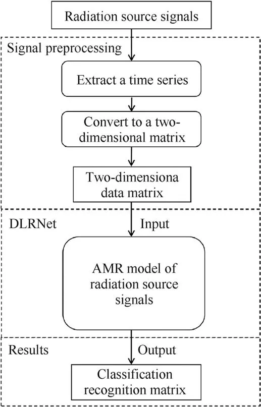
Fig.6.Automatic modulation recognition process.

The radiation source signals dataset was obtained by MATLAB simulation.In the simulation,the carrier frequencies of the various signals obtained after down-conversion are set to random values in the range of [100, 600] MHz with a step size of 100 kHz.The sampling frequency is set to ten times the carrier frequency.The SNR range of the dataset is[-20,5]dB with a variation step of 1 dB.Since a two-dimensional data matrix must contain at least one complete signal modulation period.Therefore, according to the constraint relationship between the length of the two-dimensional data matrix and the sampling rate and the signal modulation period in Eqs.(2)and(3),as well as the parameters of the signal,the length of the two-dimensional data matrix is set to L =180.A total of five datasets with consistent parameter ranges were generated, each containing 6000 samples,with approximately 857 samples for any one modulation-type signal.The total sample size of the dataset is 30,000, and the ratio of the training set to the test set is 4:1.

To verify the generalization ability and recognition accuracy of the model, a fixed SNR dataset is used for evaluating model performance.This dataset was not used for the model training process.The SNR range for this dataset is [-30,10] dB with a variation interval of 2 dB.The total number of signal samples for each SNR is 6,000,and the number of samples for different modulated signals is approximately 857.To eliminate the effect of random factors, the average of multiple test data is taken as the model test result at each fixed SNR.

The specific parameters of various radiation source signals are shown in Table 1,where CF stands for carrier frequency,MF standsfor modulation frequency,PW stands for pulse width,FD stands for frequency deviation, DC stands for duty cycle, and EW stands for code element width.

Table 1 Parameters of different radiation source signals.

The batch size and epochs used in the training process are 64 and 300,respectively.A total of 375 signal samples are included in each batch.The SGDM is used, where the SGDM learning rate is 0.0001 and momentum is 0.9.The hardware used in this paper is an Nvidia GeForce GTX 3080Ti 12 GB.

Based on the network structure of the radiation source signals modulation-type recognition model mentioned above, we constructed a DLRNet with a layered architecture and the corresponding output dimensions of each layer, as shown in Table 2.In Table 2, N represents the total number of modulation types of the radiation source signals.

4.2.Model performance analysis

The training loss curve, test loss curve, training accuracy curve and test accuracy curve generated by the model during the training process are shown in Fig.7.The loss function values and model recognition accuracy obtained for each training epoch are recorded and plotted in the figure, which visually reflects the DLRNet training process.As shown in Fig.7, the loss function value of the model decreases rapidly within 50 epochs, and the accuracy improves rapidly to approximately 80%.As the number of model training epochs increases, the value of the loss function decreases steadily, and the model accuracy gradually improves.The final overall model recognition accuracy was 93.58% on a training dataset with an SNR range of [-20, 5] dB and a variation step of 1 dB.

The trend of the training loss curve and the test loss curve shows that the DLRNet overfitting is very slight.This is also intuitively reflected in the accuracy improvement in the model, where the curves of training accuracy and testing accuracy are very close.

The confusion matrix of the model is given in Fig.8.The confusion matrix shows that DLRNet has a certain confusion interval in recognizing the radiation source signals of TRIFM and SINFM modulation types.The probability of confusion betweenother modulation-type signals is small.As shown in Figs.8(a) and(b), the model recognition results are stable for different modulation types of radiation source signals with different sample sizes.The recognition accuracy of the model is not altered by the change in the sample size.To further understand the recognition of DLRNet for each modulation-type signal during the training process.The trend of recognition accuracy with SNR for different signal modulation types are plotted in Fig.9.As shown in the figure, the recognition accuracy of two modulation types,TRIFM and SINFM,is slightly lower than that of the other signal modulation types.When the SNR is greater than-13 dB,the recognition accuracy of several other modulation-type signals is close to 100%.According to the confusion matrix and the analysis results in Fig.9, the reason why DLRNet’s recognition rate for TRIFM and SINFM modulated signals is slightly lower than other modulated signals is due to the higher similarity of these two signals.Both types of modulated signals are linear FM signals, and there is a degree of similarity in the modulated waveforms.At low SNRs, it is more difficult for DLRNet to recognize these two modulated signals.As the SNR increases,DLRNet can recognize both modulated signals effectively.When the SNR is greater than -6 dB, the recognition rate for SINFM modulation-type signals is maintained at approximately 80%.The recognition accuracy of the TRIFM modulation-type signal is above 80%, and with increasing SNR, the recognition accuracy is stable above 90%.

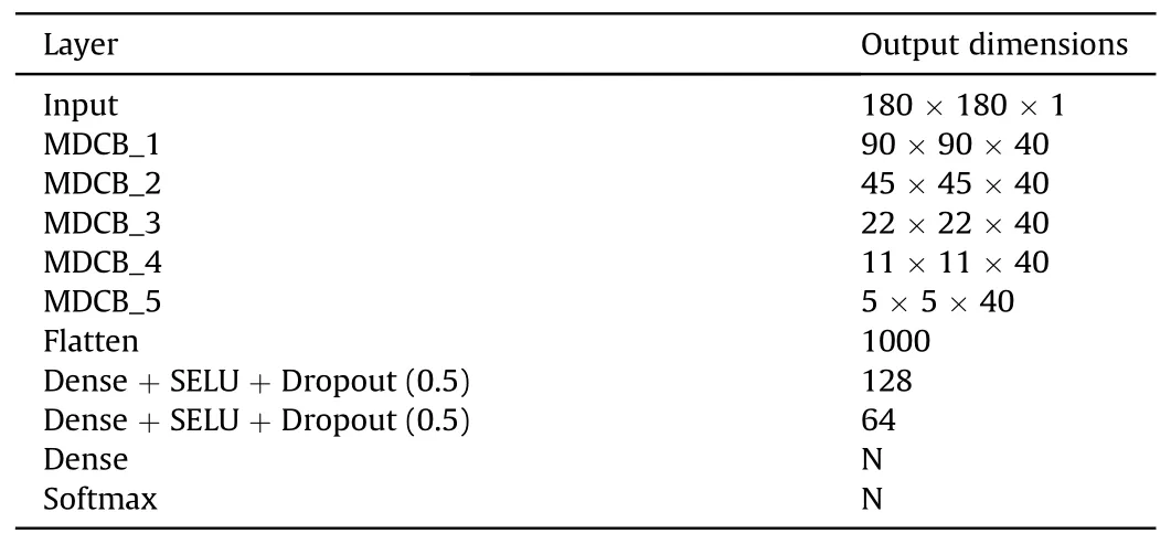
Table 2 DLRNet layer.

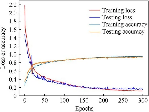
Fig.7.DLRNet model training process.The SNR of the training dataset ranges from[-20, 5] dB with a variation step of 1 dB.

From the model training results, the parameters of the AMR method of radiation source signals proposed in this paper are set reasonably, and the model structure is effective.The method can recognize multiple modulation-type signals well at a low SNR.The experimental results effectively verify the feasibility of the method in this paper for the AMR task.

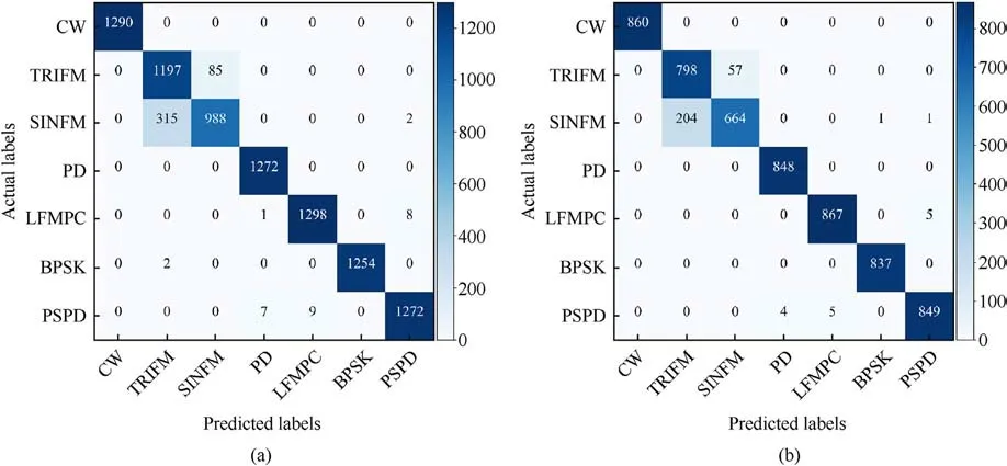
Fig.8.DLRNet’s confusion matrix for the recognition results of the signal of different modulation types: (a) and (b) show the confusion matrix with different sample sizes.

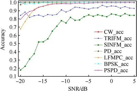
Fig.9.Curves of DLRNet’s recognition accuracy with SNR for different signal modulation types.The SNR of the dataset ranges from [-20, 5] dB with a variation step of 1 dB.

4.3.Ablation experiments

In this section,ablation experiments are used to further analyze the effect of the convolutional kernel size and different connection structures on the model performance.Starting from the ablation experiments,a dataset with an SNR range of[-30,10]dB and a step size of 2 dB was used to evaluate the model performance.

4.3.1.Convolution kernel size

In this section, the effect of the convolutional kernel size on model performance is verified by modifying the size of the convolutional kernel.The size of the convolution kernel is set to 3,5,7,9 and 11.The DLRNet model convolutional kernel size is 9.The model recognition accuracy with different convolutional kernel sizes is shown in Fig.10.

The curve with K=9 in Fig.10 is the recognition accuracy curve of DLRNet with a fixed SNR dataset.When SNR = -14 dB, DLRNet achieves 90%recognition accuracy.The accuracy of the model is still further improved as the SNR rises.The recognition accuracy of DLRNet is stable above 97% when the SNR is greater than 0 dB.

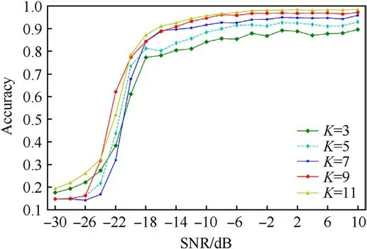
Fig.10.Recognition accuracy curves of the model with SNR for different convolutional kernel sizes.

As shown in Fig.10,the model recognition accuracy increases as the convolutional kernel size increases.When the SNR is higher than -18 dB, the large convolutional kernel is more effective in improving the model recognition accuracy.As the size of the convolution kernel increases, the computational cost of the model gradually increases.Fig.10,the curve for K=11 is very close to the curve for K=9.When the size of the convolutional kernel is equal to 9, increasing the size of the convolutional kernel does not significantly improve the model recognition accuracy.Therefore,the size of the depthwise convolutional kernel is set to 9 in DLRNet.

The experimental results verify the previously mentioned effect of convolutional kernel size on model accuracy.Large convolution kernels are more effective in handling highly random and weakly correlated data.Increasing the convolutional kernel size is beneficial for increasing the perceptual field and improving the feature extraction ability and recognition accuracy of the model.

4.3.2.Location and effect of CB

The 1 × 1 convolutional layer can perform feature extraction and information fusion.In this section, the effect of the 1 × 1 convolutional layer on the model recognition accuracy is analyzed by changing the different CB positions in the model.

The MDCB consists of a CB, two DRB and a max pooling layer cascade.The MDRB consists of only two DRB and a max pooling layer cascade.In DLRNet,the feature extraction module consists of a cascade of five MDCBs.The combination of one MDCB with four MDRBs is used in this experiment.The MDCB are positioned sequentially from the first to the fifth layer to obtain the models DLRNet_R1, DLRNet_R2, DLRNet_R3, DLRNet_R4, and DLRNet_R5.The recognition accuracy curves with SNR for the above models are illustrated in Fig.11.

As shown in Fig.11,the DLRNet_R1 and DLRNet_R2 recognition accuracy curves are closer,and the recognition accuracy at different SNRs is higher than that of the other DLRNet_Rx.The trend of the different curves shows that the closer the MDCB is to the input layer, the higher the model recognition accuracy.The position of the MDCB represents the position of the CB in the model.The closer the position of the MDCB is to the input layer,the larger the size of the image input to the CB.Combined with the above data and analysis, the larger the image size processed by the 1 × 1 convolutional layer, the more powerful the feature extraction and information fusion can be,and the more obvious the improvement in model performance.

In Fig.11, the recognition accuracy curve of DLRNet is also included.The recognition accuracy of DLRNet is significantly higher than that of all DLRNet_Rx.MDCB is used in all DLRNet models.Therefore, MDCB is effective in DLRNet.

4.4.Model recognition performance evaluation

A dataset with an SNR range of[-20,5]dB and a variation step of 1 dB is used as the training set to evaluate the performance of the AMR method of radiation source signals proposed in this paper.A dataset with an SNR range of [-30,10] dB and a variation step of 2 dB was used to test the recognition accuracy.We compare the recognition accuracy of DLRNet, ResNet-18, DenseNet-21, and the methods proposed in the Refs.[15,20].

The trend of the recognition accuracy curve of each model with the SNR is shown in Fig.12.The model recognition accuracy improves as the SNR increases.When the SNR range is [-24,-8] dB,the DLRNet recognition accuracy is significantly higher than that of the other models.When the SNR is greater than-8 dB,the DLRNet recognition accuracy reaches more than 95%.In the SNR range of[-8,10]dB,the DLRNet recognition accuracy curves almost overlap with the highest recognition accuracy curves of other models, and the recognition results are almost the same.The above analysis results show that the recognition effect of DLRNet is significantly better than that of the current mainstream AMR models.

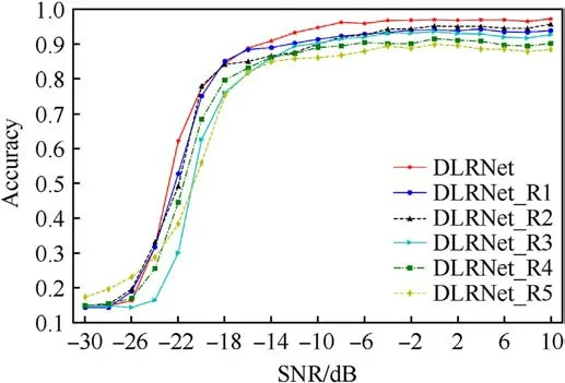
Fig.11.Curves of the variation in recognition accuracy with SNR for each model.

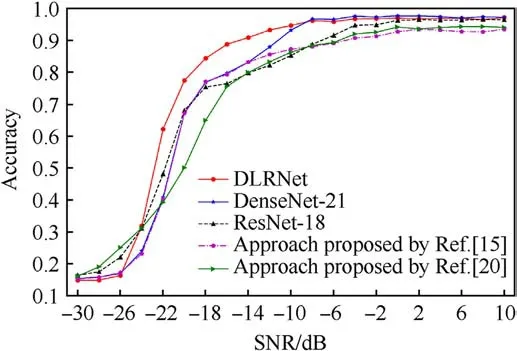
Fig.12.Curves of the variation in recognition accuracy with SNR for different models.

The DLRNet recognition accuracy for different signal modulation types during the model performance evaluation is recorded and plotted in Fig.13.The figure shows the DLRNet recognition accuracy for each modulated signal increases with increasing SNR.When the SNR is higher than -8 dB, the recognition accuracy of each modulated signal reaches more than 80%.DLRNet’s recognition accuracy for CW,PD,LFMPC,BPSK,and PSPD signals is close to 100%when the SNR is greater than-12 dB.The results further verify that DLRNet can effectively recognize the modulation types of different modulated signals at low SNRs.

As shown in Figs.12 and 13,the AMR method of radiation source signals based on two-dimensional data matrix and improved residual network can autonomously recognize multiple radiation source signals modulation types in a low SNR environment with high recognition accuracy.When the SNR reaches -22 dB, the method recognition accuracy can reach more than 60%.When the SNR reaches -18 dB, the method recognition accuracy is higher than 80%.When the SNR reaches -14 dB, the method recognition accuracy reaches 90%.

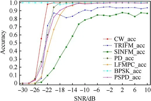
Fig.13.Accuracy curves of DLRNet recognition for different signal modulation types.The SNR of the dataset ranges from [-30,10] dB with a variation step of 2 dB.

5.Conclusions

In this paper,an AMR method of radiation source signals based on two-dimensional data matrix and improved residual neural network is proposed.The method consists of two main components.The first part is a proposed preprocessing method to reconstruct the two-dimensional data matrix by time series.By converting the time series of intercepted radiation source signals into the form of a two-dimensional data matrix, the degree of autonomy of the AMR task is increased,and the signal preprocessing process is simplified.The second part is the construction of an improved residual neural network model based on depthwise convolution and large convolutional kernels.By applying depthwise convolution and a larger convolution kernel, the feature extraction and recognition performance of the model are greatly improved.Through simulation experiments, the recognition performance of the proposed AMR method is tested in different SNRs,and compared with different methods.The results show that the proposed method can significantly improve the accuracy of the AMR method compared to other methods,especially in the case of low SNR.The recognition accuracy of the proposed method maintains a high level greater than 90% even at -14 dB SNR.

Currently, the AMR method based on two-dimensional data matrix and improved residual neural network proposed in this paper can only recognize signals of a single modulation type.And when SNR is lower than -22 dB, the recognition ability of the model decreases sharply.To further improve the recognition accuracy and effectiveness of the AMR method, our future work will focus on the modulation recognition of multiple modulation types of radiation source signals in composite scenarios, and further improve the recognition accuracy of the AMR method at lower SNRs.

Declaration of competing interest

The authors declare that they have no known competing financial interests or personal relationships that could have appeared to influence the work reported in this paper.

Acknowledgement

National Natural Science Foundation of China under Grant No.61973037 and China Postdoctoral Science Foundation under Grant No.2022M720419.