
Majorana noise model and its influence on the power spectrum
2024-01-25 07:29:42ShumengChen陈书梦SifanDing丁思凡ZhenTaoZhang张振涛andDongLiu刘东
Chinese Physics B 2024年1期
Shumeng Chen(陈书梦), Sifan Ding(丁思凡), Zhen-Tao Zhang(张振涛), and Dong E.Liu(刘东),3,4,5,†
1State Key Laboratory of Low Dimensional Quantum Physics,Department of Physics,Tsinghua University,Beijing 100084,China
2School of Physics Science and Information Technology,Shandong Key Laboratory of Optical Communication Science and Technology,Liaocheng University,Liaocheng 252059,China
3Beijing Academy of Quantum Information Sciences,Beijing 100193,China
4Frontier S
cience Center for Quantum Information,Beijing 100084,China
5Hefei National Laboratory,Hefei 230088,China
Keywords: Majorana zero mode, topological quantum computation, topological devices, decoherence and noise in qubits
1.Introduction
Non-Abelian anyons offer a novel methodology for potentially achieving fault-tolerant quantum computation,wherein quantum information is encoded using non-local degrees of freedom and quantum operations are manipulated in a manner that is topologically protected.[1–8]Of particular interest in this context are the Majorana zero modes that can be potentially hosted by topological superconductors, which are widely regarded as the most realizable candidates for topological quantum computation.[9–24]
Numerous theoretical proposals have been put forward regarding the readout and manipulation of Majorana qubits in superconducting nanowires.[23,25–42]In these designs, the qubit is encoded in a non-local manner using the parity of pairs of Majorana zero modes.In topological quantum computing,the readout of Majorana parity is of significant importance,and a number of methods have been proposed for this purpose.These include projective measurement schemes[28,29]and continuous measurement approaches with the use of quantum dot ancillaries,[26,43]as well as a conductance-based readout method in a dot-free configuration under a tunable magnetic flux.[30]A recent publication[44]briefly discusses the above different techniques used for Majorana parity readout.Among these methods,the use of quantum dot ancillaries for measurement displays considerable promise due to its scalability.[29]In work by Steineret al.,[43]a continuous measurement scheme employing quantum dot ancillaries is suggested to distinguish between Majorana parities.Specifically, the power spectrum of current correlation is utilized under the diffusion limit of a quantum point contact to achieve this objective.Building upon this idea, we examine the physical parameter discussed in Wiseman and Milburn’s work[45]and derive the power spectrum of current in the quantum point contact utilizing the quantum jump model.Based on this model,we then study a readout method for Majorana parities.It is suggested that Majorana readout based on the quantum jump model may be more practical for real materials and experimental devices.
While Majorana qubits possess certain theoretical advantages, quantum information can still be affected by both internal and external noise sources.[46–53]Therefore, refining the noise model and evaluating its impact is crucial for the progress of Majorana quantum computation.The Majorana noise model was initially developed to study the impact of noise on quantum channels by Knapp and coworkers[53]In this regard, the model was used to investigate the pseudothreshold of the Majorana qubit realization of Bacon–Shor code.To further investigate the effect of noise from a quantum dynamics perspective,we proposed a concise Majorana noise model based on the master equation in Lindblad form.We combined this model with the Majorana noise model and conducted numerical research to examine the influence of noise on the readout signal.Our study yielded insights into how different types and intensities of noise affect the power spectrum and frequency curve.Based on these findings, we developed an approach for detecting noise in the Majorana qubit.We employed a quaternion array(Γ1,Γ2,εhyb,g2)to classify the noise, while peak width, peak weight, fusion point and curve structure were used to label the frequency curve as it varied with quasi-particle poisoning rate.By analyzing the characteristics of the frequency curve,we obtained crucial information about the noise,thus introducing an approach for investigating noise in the Majorana qubit.
The present paper is structured as follows.Section 2 provides the formulation of the noise model for quasi-particle poisoning and Majorana overlapping noise based on the master equation in Lindblad form.In Section 3, we offer a comprehensive review of the Majorana parity readout technique and develop it further through the use of the quantum jump model for quantum point conduction coupled with an ancillary quantum dot.Subsequently, in Section 4, we evaluate the impact of noise on the readout signal through numerical calculations using the model presented in Section 2 and the methodology elaborated in Section 3;based on these results,we propose an approach for detecting noise in the Majorana qubit.
2.Majorana noise model
The issue of noise in Majorana qubits has been extensively discussed in previous works such as Refs.[29,46,47,50,51,53,54].As a complement to these discussions,this section presents a mathematical formulation in Lindblad form to model the effects of quasi-particle poisoning noise and Majorana overlapping with fluctuations.
2.1.Single quasi-particle poisoning event
Quasi-particle poisoning represents a major source of noise in Majorana qubits.
This phenomenon is primarily attributed to the presence of superfluous electrons within the device, as well as the ensnarement of those single electrons by the Majorana wave function.The creation of those single electrons is generally provoked by thermal excitation or radiationinduced excitement of Cooper pairs within the superconducting material.[47,53]Because quasi-particle poisoning can directly change the parity state of a Majorana qubit, it can lead to either qubit error or leakage,causing the Majorana qubit to deviate from its original computational subspace,resulting in negative impacts on the storage and retrieval of information for topological quantum bits.
In this section,we adopt the quantum trajectory approach outlined in Refs.[55,56] to construct our noise model.Our starting point is the simplest noise event,namely,a Majorana quasi-particle poisoning event, denoted as ˆγ1, that occurs in one of the Majorana zero modes.We assume that the quasiparticle poisoning rate,denoted asΓ1,remains constant and is entirely determined by the environment, i.e., independent of the system state.At timet,the quasi-particle poisoning event dN(t)=1 occurs with a probability ofp1=Γ1dtduring the time interval dt.Here,N(t) represents the number of quasiparticle poisoning events up to timet.The operator associated with this event can be expressed as
such that
Then, by the conservation of probability, we can define the operator when no event happens ˆA0by
then
Thus,we can get the state for both evolutions.For dN(t)=1,
For dN(t)=0,
Then,the stochastic Schr¨odinger equation is
Then by Ito rules and taking averageE[dN]=Γ1dt, we can get the master equation of quasi-particle poisoning
whereρMpresent the density matrix of the Majorana qubit.The noise model can also be obtained when a quasi-particle poisoning event affects the whole Majorana zero mode in the same way,
In order to obtain an estimate of the quasi-particle rateΓi,we can make use of the values reported in Refs.[47,51].These values take into account all potential sources of uncorrelated quasi-particle poisoning events that contribute toΓi.
2.2.Overlapping with fluctuation
Taking into account the finite size of nanowires,the effective Hamiltonian for the Majorana system takes the form[9,37]
Here,the value ofεhybwas discussed in Refs.[9,37,54].However, we assume that the hybridization energy may exhibit fluctuations, leading to a corresponding fluctuating Hamiltonian given by
In this expression, the termgξ(t) represents the fluctuation contribution and we assume that it follows Gaussian statistics such that
Here,grepresents the intensity of the noise and dWdenotes the Wiener increment.Using these assumptions,we can obtain the following property forδε(t):
For Gaussian white noise,
whereδ(t −τ)is the Dirac function.Then
With certain encoding, we can have iγ1γ2=σzunder a qubit basis.Then,by Ito rules,we can get the propagator
Then,by taking the average of stochastic wave function increment dρ=d(|ψ〉〈ψ|),we can get the master equation for the fluctuating hybridization energy.
So far, we have obtained the master equation for Majorana overlapping with Gaussian fluctuation.
3.Majorana parity readout by continuous measurement
Several proposals for Majorana readout methods utilizing quantum dot ancillaries have been presented in the literature.[26,28,29,57]In contrast,Steineret al.[43]introduced a novel technique that relies on continuous measurement.This method utilizes the power spectrum of current correlation in a quantum point contact, in conjunction with a quantum dot,to differentiate between different Majorana parities.A recent review article[44]provides a succinct overview of various Majorana readout approaches.We begin by introducing the effective tunneling Hamiltonian for a Majorana coupled with quantum dots[30]
The Majorana parity-dependent effective tunneling amplitude,denoted bytp,is given bytp=t1−ipt2.Alternatively,we can expresstpin terms of the phase difference betweent1andt2astp=|t1|(1−i eiθ pλ),whereλ=|t2|/|t1|andθ=Arg(t2/t1).This expression serves as the fundamental premise for all Majorana parity readout techniques that employ quantum dot ancillaries.
The article[29]discusses three methods for measuring the parity-dependent tunneling amplitude in a Majorana system.The first method involves energy-level spectroscopy,whereby the ground-state energy difference is measured.The second and third methods rely on the measurement of the differential capacitance and the average dot occupation number, respectively.
Reference [28] proposes a Majorana readout method based on the direct measurement of the parity-dependent Rabi-oscillation frequency, which originates from the paritydependent tunneling amplitude.However, this method requires a fast projective measurement of the quantum dot,which poses experimental challenges.Therefore, Ref.[43]suggests a continuous measuring approach to overcome these challenges.In this approach, the Rabi-oscillation frequency is obtained by measuring the current correlation in a quantum point contact coupled to the quantum dot ancillary.The setup for continuous measuring is shown in Fig.1.As discussed in Refs.[45,55,58–61], two models describe the current in a quantum point contact.In addition, Ref.[43] employs the diffusive model.Here,by considering the discussion in Refs.[45,62],we explore the quantum jump model as a suitable framework for simulating scenarios that involve a photon number detector.

Fig.1.Setup for continuous measurement of Majorana parity.
Subsequently, the following Hamiltonian for the perfect Majorana island connected to a quantum dot is introduced:
In the low-temperature regime and under the strong magnetic field required for a topological phase,[11,20]the effective Hamiltonian for a single spinless fermion level can be approximated for the quantum dot
whereε1is the dot level andis the particle number operator for the electron of the quantum dot.In the work by Karziget al.,[29]the charging energy terms of the quantum dot and the superconducting island are taken into consideration.By employing the parameter transformation method discussed in Ref.[57], the mutual charging energy term and the dot level term are effectively combined into a single charging energy term,which can be expressed as ˆHC+QD=εC(ˆn1−n1g)2,where ˆn1represents the particle number operator of the quantum dot andn1gis the quantum dot’s ground state occupation number.The parameterεCdenotes the effective dimensionless gate voltage of the superconductor–quantum dot system and the effective charging energy.The detailed treatment can be found in the appendix of Ref.[57].As the system operates in the resonance regime,where the energy of the quantum dot is approximately equal to the charging energy of the superconductor,for simplicity,the authors useε1as the effective tuning parameter and express the effective Hamiltonian of the quantum dot asε1ˆn1.This simplification does not affect the matrix form or the measurement result.
Subsequently, the quantum point contact is integrated as a dot occupation number monitor in the subsequent stage,enabling the extraction of parity information from the current flowing through the quantum point contact.We follow a strategy similar to that used for a double quantum dot[60,61,63,64]and obtain the dynamics for the Majorana–quantum dot setup

The Hamiltonian for the quantum point contact can be expressed as follows:
where ˆcLk, ˆcRkandωLk,ωRkare, respectively, the electron annihilation operators and the energy levels for the left and right reservoir states at wave numberk.Tkqis the tunneling amplitude for the corresponding tunneling channel.The Hamiltonian describing the interaction between the quantum dot and quantum point contact is given as
When the quantum dot is occupied,the effective tunneling amplitude of quantum point contact changes fromTkq →Tkq+χkq.Next,we follow the approach presented in Refs.[55,63]and obtain the conditional current in the quantum point contact based on the quantum jump model
The two values currently depend on the dot occupation number.The reduced two-time-correlation function is defined as
where E[]present the ensemble average.
In the general case, it is preferable to conduct numerical investigations onR(τ).However,in the case whereε1=0,an analytical expression is available, the current correlation for Majorana coupled to the quantum dot is
Then
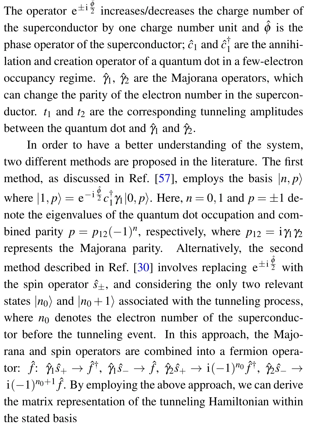
whereS0=e2(D'+D)represents the shot noise.Thus we can distinguish between different Majorana parities by the power spectrum of the current in quantum point contact.Figure 2 shows the numerical simulation of the power spectrum for different Majorana parity values.
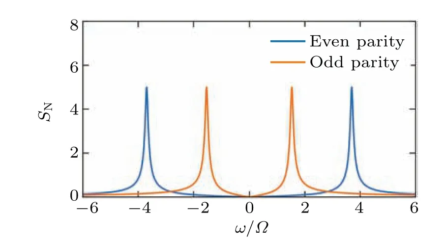
Fig.2.Power spectrum for different Majorana parity values.The normalized power spectrum, as defined here, is represented by SN =,where the parameters are specified as follows:λ =1,θ=π/4,κ =0.2|t1|,and|t1|=Ω.It is worth noting that Ω serves as the reference frequency unit here.
4.Noise influence on parity readout
The scheme presented in Ref.[43] posits a power spectrum current correlation technique for ideal Majorana qubits,featuring zero noise, as a means of Majorana parity readout.In this scenario,the current correlation can be computed from the fixed parity subspace, much akin to the double quantum dot system with a constant tunneling amplitudet1+ipt2.This approach remains valid for other parity readout methods for Majorana qubits, such as measuring the average occupation number of the quantum dot,for which only the subspace warrants consideration.Nevertheless, when probing the impact of Majorana noise, comprehensive consideration of the full Hilbert space, inclusive of both the Majorana qubit and the quantum dot,becomes indispensable.
For quasi-particle poisoning,we can get the dynamics of a Majorana coupled with a quantum dot
For Majorana overlapping,we can get
For Majorana overlapping with fluctuation,we can get
As the analytical solution to the aforementioned master equation is considerably intricate,our discussion primarily focuses on the numerical outcomes.
4.1.Quasi-particle poisoning
For quasi-particle poisoning, the following special scenarios are first considered: whenΓ1=Γ2, whenΓ1/=0 andΓ2=0, and whenΓ1=0 andΓ2/=0.The first situation describes a homogeneous environment,whereas the second and third cases represent specific instances of an inhomogeneous noise environment.This study chiefly examines three parameter regions concerning the quasi-particle rate: (1) when the quasi-particle poisoning rate is significantly smaller than the Rabi oscillation frequency,(2)when the quasi-particle poisoning rate is of the same order of magnitude as the Rabi oscillation frequency,and(3)when the quasi-particle poisoning rate is much greater than the Rabi oscillation frequency.
In the context of homogeneous quasi-particle poisoning noise, we can denote the noise intensity byΓ=Γ1=Γ2.As demonstrated in Fig.3(a), when the quasi-particle poisoning rate is very small (Γ ≪|t1|), the peak frequency exhibits an insignificant shift.This indicates that the parity measurement result can be obtained with high precision under such a noise intensity.As the quasi-particle poisoning rate increases, the two peaks move towards each other, accompanied by an increase in peak width,and eventually merge into a single peak at the Rabi oscillation frequency(Γ ≈|t1|).This implies that,in this range, the two peaks cannot be distinguished and the Majorana parity cannot be obtained from the measurement.As the quasi-particle rate further increases, the merged peak shifts its frequency to zero.This implies that when the quasiparticle poisoning rate is much larger than the Rabi oscillation frequency,the current in QPC is described by shot noise,which is similar to the behavior observed in coupled quantum dots whenκ ≫4Ω.Here,κ=|˜χ|2represents the coupling strength between the quantum dot and QPC,andΩrepresents the coupling strength between quantum dots.In this case,the electron will be localized in the quantum dot, a phenomenon also referred to as the quantum Zeno effect.Figures 3(b)–3(d)illustrate the power spectrum at different levels of noise intensity.
Subsequently, an observation was made that the power spectrum’s structure changes in the presence of quasi-particle poisoning.As depicted in Figs.4(a) and 4(b), a secondary peak emerges at the location of the opposite parity with a comparatively smaller weight for each parity.Here, weight corresponds to the area enclosed by the corresponding peak.The secondary peak remains negligible under a relatively low quasi-particle poisoning rate but becomes noticeable at a magnitude proximate to the Rabi frequency.As the noise intensity rises, the weight of the secondary peak increases.The primary and secondary peaks merge into a single peak with an increase in noise intensity.This phenomenon is attributed to the quasi-particle poisoning event’s alteration of the Majorana parity and the effective tunneling amplitude,resulting in the emergence and amplification of the secondary peak.The double-peak configuration of the power spectrum with a noise intensity ofΓ/Ω=0.5 is visually demonstrated in Fig.4(c).
Subsequently,we present a discussion on inhomogeneous quasi-particle noise.Firstly, we consider the special cases whereΓ1/= 0 andΓ2= 0, as well asΓ1= 0 andΓ2/= 0.These cases correspond to the scenario where only one Majorana zero mode undergoes a quasi-particle poisoning event.Forλ=1, the power spectrum is indistinguishable betweenΓ1/= 0,Γ2= 0 andΓ1= 0,Γ2/= 0.By comparing Figs.5 and 3, the most conspicuous dissimilarity between inhomogeneous quasi-particle noise and homogeneous quasi-particle noise is that for noise intensities much greater than the Rabi oscillation frequency;the fused frequency tends to zero in the former,whereas it tends to|t1|(also equal to|t2|)in the latter.

Fig.3.(a)Peak frequency curve of different parity under quasi-particle noise intensities(Γ/Ω)ranging from 10−3 to 101,with λ =1,θ =π/4,κ =0.002|t1|, and |t1|=Ω.The corresponding Rabi oscillation frequency,denoted as ωR,is associated with the peak.The error bar in the figures represents the peak width and the main peak of each parity state is shown.The values of κ and θ are held constant throughout the remaining images.(b) Power spectrum for Γ/Ω =0.01.(c) Power spectrum for Γ/Ω =1.6.(d)Power spectrum for Γ/Ω =10.

Fig.4.(a) Peak frequency curve for even parity under quasi-particle noise intensity ranging from 10−3 to 101,where the color bar presents the relative weight of the peaks.(b)Peak frequency for odd parity under quasi-particle noise intensity ranging from 10−3 to 101.(c)Power spectrum for Γ/Ω =0.5.

Fig.5.(a) Peak frequency curve under the influence of quasi-particle noise with intensity represented by Γ1/Ω, which varies from 10−3 to 101.Additionally, Γ2/Ω =0 and the value of λ is set to 1.The frequency diagram exhibits symmetry across the ωR =0 axis.Therefore, in (a), to provide a clearer demonstration, we only display even parity for ωR >0 and only odd parity for ωR <0.Otherwise, the even and odd parity would overlap, decreasing the picture’s clarity.(b) Peak frequency curve under the influence of quasi-particle noise with intensity represented by Γ2/Ω,which varies from 10−3 to 101, while Γ1 =0 and λ =1.Similar to (a), only odd parity is presented for ωR >0 and only even parity for ωR <0 to enhance clarity.Due to the symmetry of the frequency diagram by the axis ωR=0,(a)and(b)are identical.(c)Power spectrum for Γ1/Ω =0.5.
By comparing Figs.5 and 3,we observe the difference between inhomogeneous quasi-particle noise and homogeneous quasi-particle noise,but we are unable to differentiate between a single quasi-particle ˆγ1(Γ1/=0,Γ2=0),and a single quasiparticle, ˆγ2(Γ2/=0,Γ1=0).This lack of distinction is expected because atλ=1, the Majorana modes ˆγ1and ˆγ2possess full symmetry and thus it is not possible to distinguish between them.If we desire to distinguish between ˆγ1and ˆγ2in real space, we can set|t1|/=|t2|and break the symmetry between the noise effects ofΓ1andΓ2.For instance,whenλ=0.5,that is|t1|=2|t2|, we can define ˆγ1and ˆγ2in real space, resulting in different spectra for the two types of noise.Additionally,in the high noise region(i.e.,≥101),single quasi-particle noise exhibits distinct behavior from homogeneous quasi-particle noise: the Rabi-oscillation frequency no longer tends to zero but converges to 2|t1|forΓ2=0 and to 2|t2|forΓ1=0.
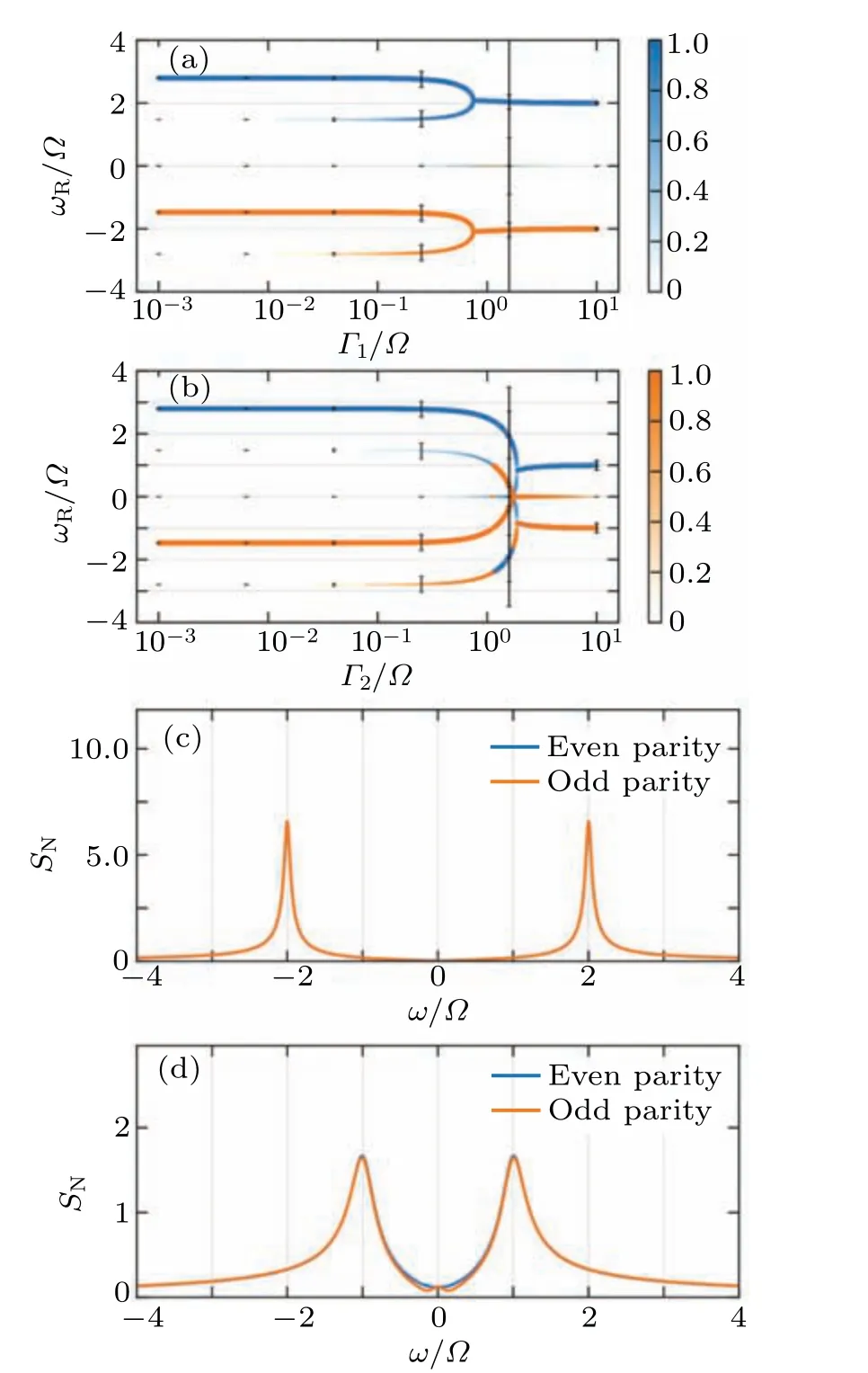
Fig.6.(a) Peak frequency curve under the influence of quasi-particle noise with intensity represented by Γ1/Ω, which varies from 10−3 to 101.Additionally,Γ2/Ω =0 and the value of λ is set to 0.5.For the sake of enhancing visual clarity, only the width of the peak with a weight greater than 10−3 is displayed and only odd parity is displayed for ωR >0.Both parities have the same configuration but with different weights, both are symmetry curves along axis ωR=0 as displayed in Figs.4(a)and 4(b),to have a better comparison,only half of each parity is displayed.(b)Peak frequency curve under the influence of quasi-particle noise with intensity represented by Γ2/Ω, which varies from 10−3 to 101.Additionally, Γ1/Ω =0 and the value of λ is set to 0.5.(c) Power spectrum for Γ1/Ω =10 Here the curve of even parity is almost covered by the curve of odd parity,since they have the same configuration.This situation is the same for(d)and other figures.(d)Power spectrum for Γ2/Ω =10.
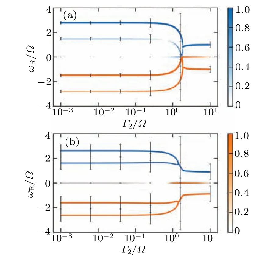
Fig.7.(a) Peak frequency curve under the influence of quasi-particle noise with intensity represented by Γ2/Ω, which varies from 10−3 to 101.Additionally,Γ1/Ω =0.1 and the value of λ is set to 0.5.(b)Peak frequency curve under the influence of quasi-particle noise with intensity represented by Γ2/Ω,which varies from 10−3 to 101.Additionally,Γ1/Ω =0.5 and the value of λ is set to 0.5.
Subsequently, we explore the case where bothΓ1andΓ2are non-zero and not equal.Specifically,we consider the range ofΓ1/Ωto be between 10−3and 101, whileΓ2remains constant.Moreover, we can setΓ1=x+C1withx ∈[10−3,101]andΓ2=C2, or conversely,Γ2=x+C2withx ∈[10−3,101]andΓ1=C1, following the approach proposed in Ref.[52].This yields the possibility of discerning the prevailing quasiparticle noise situation(represented byC1andC2)in the Majorana qubit by observing different behaviors of the power spectrum concerning the variablex.As such, we present a method for detecting noise in the Majorana qubit, with the numerical results serving as a reliable reference for experimental investigations.We demonstrate the peak frequency diagram as an illustrative example in Figs.7(a) and 7(b).Notably, distinct quasi-particle poisoning leads to different behaviors ofωR.Specifically, the peak width forΓ1/Ω=0.1 is considerably narrower than that ofΓ1/Ω=0.5 at the sameΓ2value.Both peak widths increase withΓ2before the fusion point, corresponding to the rising dissipation effect proportional to the total noise rate (Γ1+Γ2).Additionally, we observe that the fusion points for different noise intensities also differ.We denote the fusion point asF= (ΓF,ωRF),with the value ofΓFforΓ1/Ω=0.5 being larger than that forΓ1/Ω=0.1,and the value ofωRFforΓ1/Ω=0.5 being greater than the value forΓ1/Ω=0.1.Furthermore,forΓ1/Ω=0.1,the frequency curves approach zero before fusing,whereas forΓ1/Ω=0.5,the frequency curve fuses directly,indicating different fusion points.The weight of the secondary peak forΓ1/Ω=0.5 is also greater than the weight of the secondary peak forΓ1/Ω=0.1.Overall, the fusion point, peak width and peak weight serve as reliable indicators for distinguishing different noise types and intensities.Therefore,the theoretical results presented in this study can aid in detecting noise in the Majorana qubit.
4.2.Overlapping with fluctuation
This section explores the effects of overlapping and fluctuations on the power spectrum of the Majorana readout.Firstly, we analyze the impact of pure Majorana overlapping.The Hamiltonian governing the coupling between a Majorana mode and a quantum dot under the particle number basis,with pure Majorana overlapping,can be expressed as
Based on the Hamiltonian derived earlier,it is evident that pure Majorana overlapping introduces a 2εhybenergy level space,as expected.The even parity and odd parity of the Majorana are denoted as|0〉tand|1〉t,respectively.In an infinitely long nanowire,ideal zero energy degeneracy can be achieved,where the energy level for|0〉tand|1〉tis zero.However,Majorana overlapping leads to a splitting of the degenerate energy level, where the energy level for|0〉tis−εhyb, and for|1〉tisεhyb.Denoting|0〉 and|1〉 as the dot occupation number of the quantum dot, we use|01〉to represent|0〉⊗|1〉t.The energy level for|01〉 isεhyb, for|10〉 it is−εhyb, for|00〉 it is also−εhyband for|11〉 it isεhyb.Therefore, the diagonal elements of the matrix can be obtained.The effective Rabi oscillation frequency can be calculated asIt is observed that forεhyb<10−1,pure Majorana overlapping has a negligible influence.Forεhyb≥1, the peak frequency increases almost linearly withεhyband the distance between the two parities decreases, while the peak width remains almost unchanged.This indicates that pure Majorana overlapping causes minimal dissipation,which is in accordance with expectations, as illustrated in Fig.8(a).The influence ofεhybon the power spectrum can be observed from Fig.8.Asεhybincreases, the weight of the Rabi oscillation peak decreases while the weight of the zero-frequency peak increases.This indicates that Majorana overlapping leads to the shot noise effect.It should be noted that the main difference between pure Majorana overlapping and Majorana overlapping with fluctuation is the width of the peak,which is caused by fluctuation.
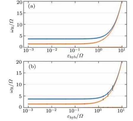
Fig.8.(a) Peak frequency curve for the scenario of pure Majorana overlapping.It is notable that the diagram possesses a symmetry with respect to ωR=0;therefore,solely the portion corresponding to ωR ≥0 is depicted.(b) Peak frequency curve for Majorana overlapping with fluctuation g2=0.1εhyb.
In Subsection 4.2, the frequency behavior of overlapping and quasi-particle poisoning noise is discussed by varying the quasi-particle injection rate.The proposed approach suggests that the noise in the Majorana qubit can be uniquely identified and labeled by a quaternion array consisting of(Γ1,Γ2,εhyb,g2), which we refer to as the characteristic array for noise.By analyzing the peak width, fusion point,frequency under the quasi-particle poisoning rate limit and curve structure of the frequency curve, we can describe the behavior of the frequency curve.The establishment of a map between the characteristic array for noise and the frequency curve enables theoretical simulations to provide valuable guidance for the detection and characterization of noise in Majorana qubits.In Fig.9,a comparison is made between different noise parameters.It is observed that, withεhyb/Ω=1, the frequency under a low quasi-particle poisoning rate is higher than the case without Majorana overlapping.Additionally,differences in peak width and weight are visible for Majorana overlapping noise with and without quasi-particle poisoning(Γ2/Ω=0.5)under a low quasi-particle poisoning rate(Γ1/Ω ≪1).ForΓ1/Ω ≈1, it is found that, before fusion,the primary peak frequency decreases but does not reach zero forεhyb/Ω=1,g2=0.1εhyb, whereas it does reach zero forεhyb/Ω=1,g2=0.1εhyb,Γ2/Ω=0.5.After fusion, the primary and secondary peaks are in the fused state forεhyb/Ω=1,g2=0.1εhyb,but forεhyb/Ω=1,g2=0.1εhyb,Γ2/Ω=0.5,there is a non-vanishing space between the primary and secondary peaks.While the physical mechanisms underlying these complex curve behaviors are still not fully understood,the differences between the curves offer a promising approach to identifying and characterizing noise in Majorana qubits.
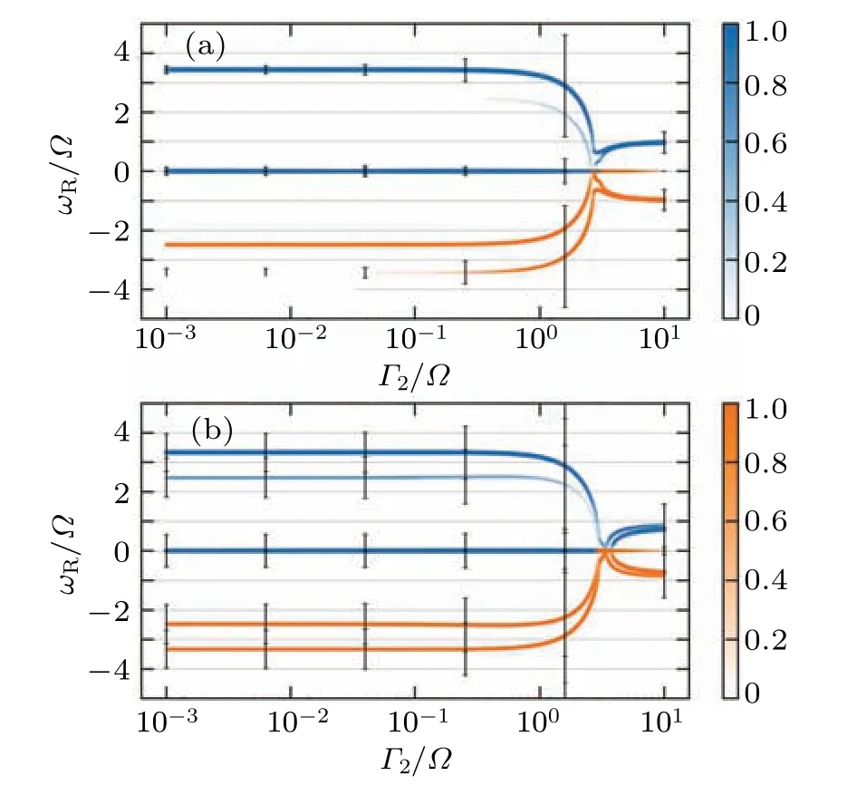
Fig.9.(a) Peak frequency curve for εhyb/Ω =1, g2 =0.1εhyb and λ = 0.5.(b) Peak frequency curve for Γ2/Ω = 0.5, εhyb/Ω = 1,g2=0.1εhyb and λ/Ω =0.5.
5.Summary and outlook
In this paper, we present a comprehensive analysis of noise in Majorana qubits, wherein we construct a Majorana noise model that incorporates quasi-particle poisoning and Majorana overlapping with fluctuation.Subsequently,we develop a method for continuous Majorana parity measurement,which relies on the quantum jump model.Furthermore, we examine the impact of noise on the readout signal and propose a new approach for detecting the noise situation in Majorana qubits.Our future work aims to expand upon our current findings and refine the mapping between noise parameters and signal curve characteristics,thereby enhancing the rigor of the Majorana noise detection method.
Acknowledgements
We would like to express our gratitude for the valuable discussions with Li Chen, Feng-Feng Song, Gu Zhang and Zhenhua Zhu.This work was supported by the Innovation Program for Quantum Science and Technology (Grant No.2021ZD0302400), the National Natural Science Foundation of China (Grants No.11974198), and the Natural Science Foundation of Shandong Province of China (Grant No.ZR2021MA091).
猜你喜欢
摄影之友(2022年10期)2022-10-22 02:15:48
摄影之友(2022年6期)2022-06-30 13:54:00
阅读(低年级)(2022年5期)2022-06-03 14:01:10
阅读(低年级)(2022年4期)2022-06-02 07:43:55
剧影月报(2019年6期)2019-11-15 18:48:34
动漫星空(2018年4期)2018-10-26 02:11:58
微型小说选刊(2015年10期)2015-11-17 17:15:06
小天使·一年级语数英综合(2014年4期)2014-04-09 07:10:28
飞天(2009年6期)2009-09-02 01:46:04
故事会(2008年14期)2008-01-06 10:18:44

- Chinese Physics B的其它文章
- High responsivity photodetectors based on graphene/WSe2 heterostructure by photogating effect
- Progress and realization platforms of dynamic topological photonics
- Shape and diffusion instabilities of two non-spherical gas bubbles under ultrasonic conditions
- Stacking-dependent exchange bias in two-dimensional ferromagnetic/antiferromagnetic bilayers
- Controllable high Curie temperature through 5d transition metal atom doping in CrI3
- Tunable dispersion relations manipulated by strain in skyrmion-based magnonic crystals