A Monte Carlo Lagrangian Droplet Solver with Backpropagation Neural Network for Aircraft Icing Simulation

，，，3*，，3

1.Low Speed Aerodynamic Institute， China Aerodynamics Research and Development Center， Mianyang 610082，P.R.China； 2.Anti/De-Icing Key Laboratory， China Aerodynamics Research and Development Center，Mianyang 610082， P.R.China； 3.Key Laboratory of Aerodynamics， Mianyang 610082， P.R.China；4.School of Computer Science， Southwest Petroleum University， Chengdu 610500， P.R.China

Abstract: In-flight icing is threatening aviation safety.The Lagrangian method is widely used in aircraft icing simulation to solve water collection efficiency， the development of which has been impeded by robustness issues and high computational cost.To resolve these disadvantages， two critical algorithms are employed in this study.The Monte Carlo integral method is applied to calculate collection efficiency， which makes the Lagrangian method unconditionally robust for an arbitrary situation.The backpropagation（BP） neural network is also implanted to make a rapid prediction of droplet impingement.Additionally， these two algorithms are deeply coupled in an asynchronous parallelism that allows un-interfered parallel for each procedure respectively.The current study is implemented in NNW-ICE software platform.The asynchronous solver is evaluated with a 3D GLC-305 airfoil and a jet engine nacelle model.The result shows that the BP network contributes a significant acceleration to the Monte Carlo method， saving about 27% running time to achieve equal accurate result.The study is a first attempt for coupling the neural network art and numerical simulation in aircraft icing， providing strong support for the improvement of Lagrangian method and aircraft icing.

Key words：aircraft icing； Lagrangian method； Monte Carlo method； backpropagation（BP） neural network；asynchronous parallelism

0 Introduction

The in-flight icing phenomenon is considered highly dangerous for aircrafts［1］.The supercooled droplets amongst high-altitude clouds will freeze on impact at the leading edge of wings， tail， engine nacelle， etc.The accretion of ice can lead to degradation in aerodynamic performance， and in extreme cases， even catastrophic consequences［2-3］.

Numerical techniques had been studied during the past decades to simulate in-flight icing.However， the phenomenon of icing is complicated due to the participation of multiple physical processes.Therefore， a hypothesis is made that the in-flight icing is a quasi-steady process.Such that the simulation is accomplished by four loosely coupled sub-processes： The simulation of airflow field， the simulation of droplets impingement， the simulation of energy equilibrium of icing， and the grid adaption.

The simulation of droplet impingement is the foundation of further simulations.Simulation methods are currently diverged into two primary branches， the Lagrangian method and the Eulerian method［4］.The advantages of Lagrangian method are the fidelity of physics in simulation of droplets behavior and the convenience to couple with other physical models， like droplet thermal equation， the deform and break-up model for supercooled large droplet（SLD）， and etc.The Lagrangian method has been branched by difference scheme and techniques.Typically the bin method［5］and the flow tube method［6］are widely adopted in research and industry， but mostly in 2D cases.Recent progress in Lagrangian method， proposed by Wang et al.［7］， is to merge the features of Eulerian method and Lagrangian method by solving Lagrangian concentration differential equation（LCDE）.The Lagrangian parcel volume（LPV） method was invented as a modification version of LCDE method， proposed by Triphahn［8］and Mickey et al［9］.Presently， no industrial application has been found using LCDE or LPV methods， and they need further validation on various models.

The development of Lagrangian solver is highly constrained by the robustness issue and computational cost in 3D cases.For years， the flow tube method was popularized with NASA’s LEWICE［10］code.Leading that， a group of similar Lagrangian droplet solvers were developed around 2000［11］.But the limitation was reached when encountered by complex geometry.Trials have been conducted to overcome the robustness issue.Recent evidence shows that a new Lagrangian method involving statistics was adopted in NASA’s next generation icing code GlennICE［12］and ONERA’s ONICE3D icing software［13］.Obviously， the Monte Carlo method［14］is referred to make statistic integral on calculating the surface collection efficiency.The Monte Carlo Lagrangian solver is inherently capable of solving unsteady problems， coupling with SLD models，and most importantly adapting the complex geometry.A Monte Carlo Lagrangian solver has been integrated in NNW-ICE software， developed by China aerodynamic research and development center（CARDC）.

On the one hand， the robustness issue is inherently solved by random statistics.On the other hand， the computational cost is further increased by using Monte Carlo Lagrangian solver.Therefore，the artificial neural network （ANN） technique is adapted to reduce the cost.The ANN shows huge aptitude for fast prediction and solving non-linear systems.Recently， the integration of computational fluid dynamics （CFD） and machine learning achieve great success in solving typical problems， indicating that a similar research approach is available for aircraft icing simulation.Ogretim et al.［15］proposed an ice shape prediction model applying the generalized regression neural network （GRNN） and the multilayer perception network （MLP）， respectively.The ice shape feature is transmitted by Fourier series decomposition.Similar research followed by Zhang et al.［16］contributed an improved ice shape extraction technique， and also by Chang et al.［17］using wavelet packet transform instead of Fourier series decomposition to achieve better prediction on Glaze ice.Convolutional neural network（CNN） techniques were applied by He et al.［18］and Strijhak et al.［19］respectively， using ice shape images as samples.Recently， Yi et al.［20］established strong correlation between ice shape feature and numerous numerical results on NACA0012， using backpropagation （BP）neural network.Thereafter， Qu et al.［21］expanded the prediction scope from single airfoil to arbitrary symmetric airfoil based on deep learning and multimodal fusion technique.Applications of ANN on aircraft icing simulation currently focus on fast ice shape prediction.The quantity requirement on training samples has limited the usage of ANN in 3D cases， since the experimental or numerical cost is huge.

In this paper， a Monte Carlo Lagrangian droplet solver accelerated by a parallel BP neural network is introduced.The BP neural network is employed to reduce the redundant calculation of nonimpinged droplets in Lagrangian solver.The general idea of such asynchronous solver structure will be firstly discussed.Then the Monte Carlo Lagrangian method and its improvement with the BP neural network will be introduced.Lastly， the validations on Monte Carlo method， the BP network and the asynchronous solver will be presented.

1 Algorithms

The idea behind constructing an asynchronous solver is to enable un-interfered parallelism for both the Lagrangian solver and the BP network.On the one hand， the Monte Carlo method is a statistical method， a great number of droplets are required for the algorithm to converge.On the other hand， the BP network can make impressively fast prediction of the droplet impingement result， but requires training by a great number of samples.The purpose of accelerating Monte Carlo Lagrangian droplet solver with BP neural network should not be considered satisfying if the procedure is “simulation first， prediction follows”.

Fig.1 Conceptual diagram for the asynchronous solver

Asynchronous parallelism is made by two groups of threads dealing with tasks individually.Two synchronization points are assigned for data transfer， one for the sample delivering from the Monte Carlo Lagrangian solver to the BP network and the other for the impingement prediction from the BP network to the Monte Carlo Lagrangian solver.The general idea is presented in Fig.1 and it will be discussed in detail later.

The asynchronous solver is made to overcome the disadvantage of Lagrangian method.In order to make better understanding of it， the Monte Carlo integral method and the BP neural network will be firstly revealed in this chapter.

1.1 Monte Carlo Lagrangian method

1.1.1 Governing equation and discretization

The governing equation of the Lagrangian method is established by the momentum law.The equation is solved with stationary airflow background， and the interaction between droplets and air is ignored.Some important hypothesis is made that droplets with the diameter less than 40 μm are considered as a rigid spherical body， the rotation and the collision of droplets are neglected because the icing environment is the dilute flow.The governing equation is

whereupis the velocity vector of the water droplet，uathe velocity vector of the airflow field，gthe acceleration due to gravity，ρathe density of air，ρpthe density of the water droplet， andF·(up-ua)the aerodynamic force acting on the water droplet.Fis the aerodynamic force coefficient given by

wheredpis the diameter of the droplet，Cdthe drag coefficient，Rerthe relative Reynolds number based on the droplet diameter， andμathe viscosity of air.Cdis calculated by Schiller and Naumann’s equation［22］

The governing equation is discretized by a second-order accurate Langrage exponential tracking scheme［23］

whereτpis the relaxation time defined as

1.1.2 Calculation of collection efficiency

Collection efficiency is a non-dimensional character describing the amount of water collection.The collection efficiency is defined as the portion of actual mass flow rate on surface to that of the maximum flow rate.

where the subscript “s” is an arbitrary unit surface element， andmˉsthe actual mass flow rate（kg/s） on the unit surface.

In the Monte Carlo method， on contrary to other Lagrangian method where the mass rate is transmitted to impinged area or impinged numbers， the surface mass flow rate can be inherently calculated by assigning each droplet with certain mass rate.The Monte Carlo integral method is applied on surface to calculate the mass rate， and the collection efficiency is therefore defined in Monte Carlo method as

whereMsis the total mass collected during Δttime，LWC the liquid water content describing the water density in far field space， andAsthe surface element area if using finite volume grid.

1.1.3 Solving procedure

The solving procedure is presented in Fig.2.The droplets are solved with OpenMP parallel in NNW-ICE software.

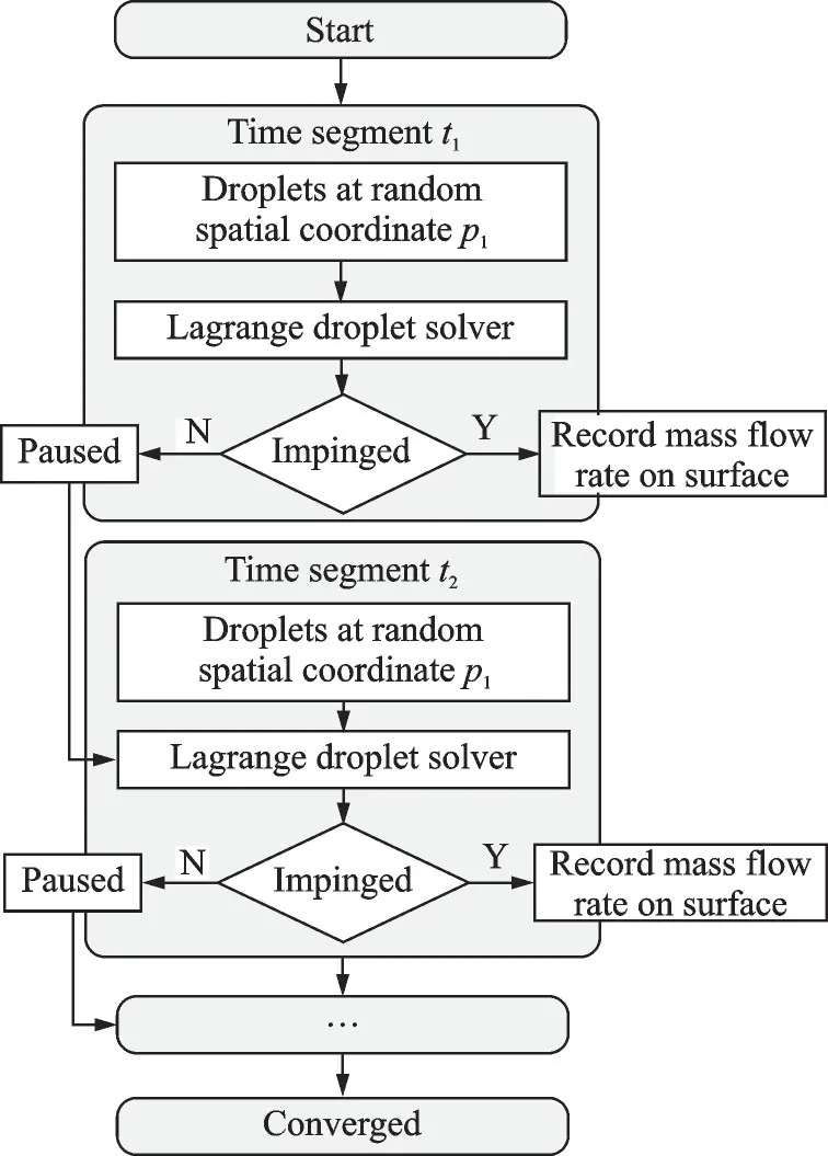
Fig.2 Solving procedure of Monte Carlo Lagrangian method

The procedure is divided into several time segments of random physical time interval.Random numbers of droplets at random positions are released at each time segment.All segments are summed up to a targeted total time， and the droplets are summed up to a target number.Each droplet is assigned with equivalent mass flow rate which summed up to far field LWC condition.Droplets are solved during each time segment according to the governing equation with tiny time step dtin Eq.（1）， advancing the physical time till the end of current segment.Impinged droplets are used for Monte Carlo integral method according to Eq.（7） to calculate the collection efficiency.Droplets that are still moving pause until next time segment starts.The statistical convergence will be reached by repeating such a procedure in each time segment successively.

1.2 Backpropagation neural network

1.2.1 The BP network structure

The BP network used in this paper has three hidden layers， one input layer with three neurons and an output layer with single neuron， comprising a structure of 3×4×4×2×1， shown in Fig.3.

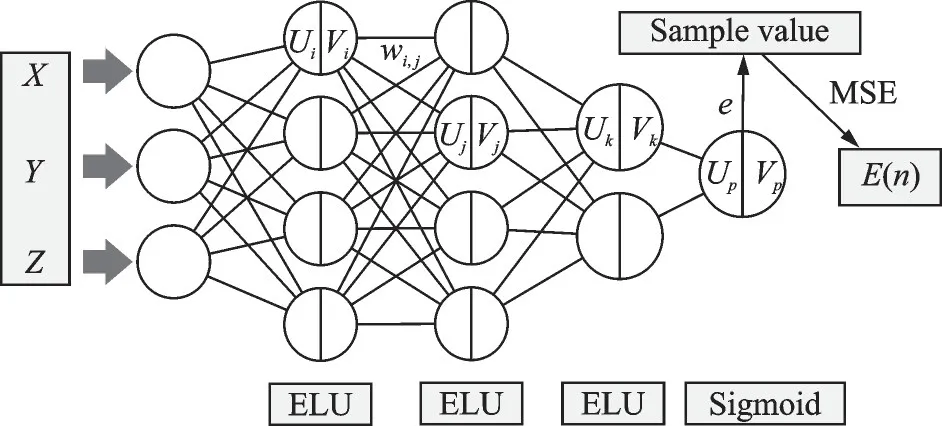
Fig.3 Structure of the backpropagation neural network

The hidden layers utilize the exponential linear unit （ELU） as activation function to avoid vanishing gradient problem.The ELU function allows for faster convergence and reduces the likelihood of an insignificant weight adjustment.Additionally， the function has a negative region that produces sparse activations， helping preventing overfitting problem.A sigmoid function is employed on the output layer to restrict the confines of network output to interval［0，1］.The network error is defined by mean square error （MSE） function.

The primary objective of this study is to predict whether or not a droplet released at a given spatial coordinate will impinge on the target surface.The constitution of such network will take a 3D coordinate as input and the probability of impingement as the output.

The gradient descent method is adopted for ease of BP training.The momentum BP method and the variable learning technique are used to improve the convergence.

1.2.2 The gradient descent method

The gradient descent method is a widely used optimization algorithm in the BP neural network.The objective for BP network is to minimize the error function （or loss function） by adjusting the weights and biases of fully connected neurons.The gradient descent algorism works by computing the gradient of error function with respect to each weight and bias， then updating them in the opposite direction to reach the minimum error along a quickest path.The local gradient of output neuronpat current iteration can be solved by the chain rule of derivative as

whereE=1/2e2is the total error defined by MSE function，e=V*p-Vpthe deviation to sample value，Upthe neuron input，Vpthe neuron output（or the activation level）， andfpthe activation function.The time denote is neglected for simplification.

The local gradient is then calculated by forward linked neurons.

whereKis the total number for current layer， andwjkthe weight from neuronjto neuronk.Arbitrary weight adjustment can be then calculated by

whereηis the learning rate.According to the chain rule of derivative， the bias adjustment is mostly the same to weights， only in absent of activation term.

1.2.3 Momentum BP method［24］

The momentum BP （MBP） method is an extension of standard BP algorithm.A momentum term is incorporated to accelerate the convergence.The adjustment for weights and biases are influenced by both the current error gradient and the accumulated gradient from previous iterations.The momentum term enables the algorithm to move smoothly along the error surface and overcome local minima to reach the global minimum efficiently.The momentum term is applied as

The superscript is denoted for training time step， andαthe momentum term.The weight adjustment of current iterationNis weight balanced by the previous matrix and the current error gradient.The momentum term is set to 0.5 to make equivalent influences from current and previous iteration.

1.2.4 Variable learning rate［25］

The variable learning rate algorithm is another modification of standard BP.This algorithm allows for variation during iteration， judged by certain features of the network.In this study， the most instinctive algorithm is employed by comparing the total error of all validation samples at the current iteration and the previous one.When the total error decreases， it is indicated that the weight adjustment is correlated to gradient path， thus increasing the learning rate to accelerate convergence.The total error increasement indicates overfitting， therefore the learning rate is to be decreased for smoother convergence.The learning rate is set 0.01 initially and the variation is restricted in ［0.001，1］ range.

Notion that the learning rateηis applied in Eq.（10） as a relaxation for gradient descent speed，and the total lossEis applied in Eq.（8）.Such relaxation of variable learning rate in Eq.（12） is substituted to Eq.（10） in each iteration.

2 Asynchronous Lagrangian Solver

The BP network can effectively predict the droplet impingement probability.A well-trained network can save considerable computation cost for certain model.However， if the prediction always comes after the simulation， it is of little significance for industrial application.The NNW-ICE software aims to solve icing and anti-icing problems in aviation and other related industries.It is necessary to further enhance the integration between the BP network and the NNW-ICE code.Therefore， The asynchronous Lagrangian solver is proposed to parallelize the Monte Carlo statistics and BP network training， thereby enabling faster predictions during simulation.

The asynchronous programing is conducted using OpenMP API.The solving procedure is depicted in Fig.4.The solver starts with limited threads pool， which is then distributed to two paralleled tasks： The Monte Carlo Lagrangian solver and the BP neural network， respectively.The droplets’trajectories are solved in the Monte Carlo Lagrangian solver at each non-uniform random time segment.Each time segment contains several time steps.The iteration of each droplet will stop at impingement or pause at the end of current time segment.The BP network starts training with samples from the Lagrangian solver.Samples will be updated at end of time segment， and previous samples are not reserved.Once the droplets all stop or pause， the first synchronize point is met.The droplets information is delivered to BP network as a new group of samples for further training.A shared tag is activated to stop the undergoing training， immediately， and the replace the outdated samples with new group.Before launching the next time segment， a group of droplets with random positions is generated.As long as the total error of BP network descents to given threshold，the second synchronize point is met.The simulation and training halt， meanwhile the prediction is conducted for newly generated droplets.Droplets that are predicted as no impinging will be neglected， only those with possibility of impingement will be calculated.

Fig.4 Running procedure for asynchronous Lagrangian solver

A confidence coefficient of 10% is selected for predicted probability， which means droplets with lower prediction result will not be calculated.This will label around 50% of droplets as “non-impinged” at relative rough training， and the labled number will grow up to 80% while the total error constantly decreases.The confidence coefficient could be adjusted as training converges.But the adjustment requires pre-experience judgment and is not generally effective for different models.

The synchronize point is realized by implanted OpenMP parallel lock， which is mutually exclusive to ensure correct data exchange.

3 Validations on Numerical Method

3.1 Validation on Monte Carlo Lagrangian solver

Numbers of cases have been validated by NNW-ICE， including classical 2D NACA65-415，MS317， GLC-305， and so on.， and 3D swept wing， engine nacelle and half-model airplane.The validation results are revealed partly in Figs.5—7.All calculation conditions are annotated on graphics.

The 2D cases are all compared with NASA’s experimental result and the LEWICE numerical result［26］.The error band of 10% is labeled on curves in 2D cases.Thex-coordinate is non-dimensional length of curve distance to airfoil chord.They-coordinate is collection efficiency.

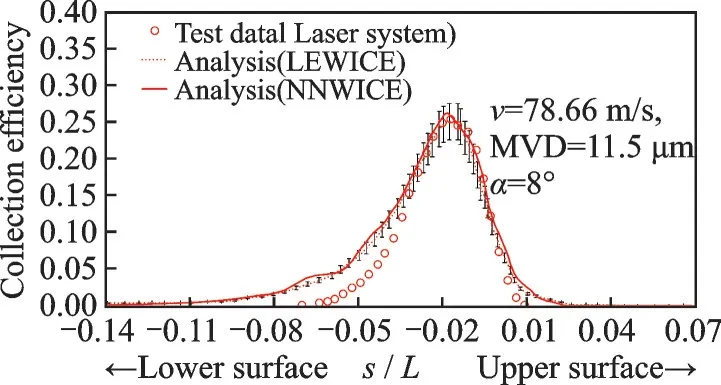
Fig.5 Validation on 2D MS317 case

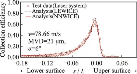
Fig.6 Validation on 2D GLC-305 case

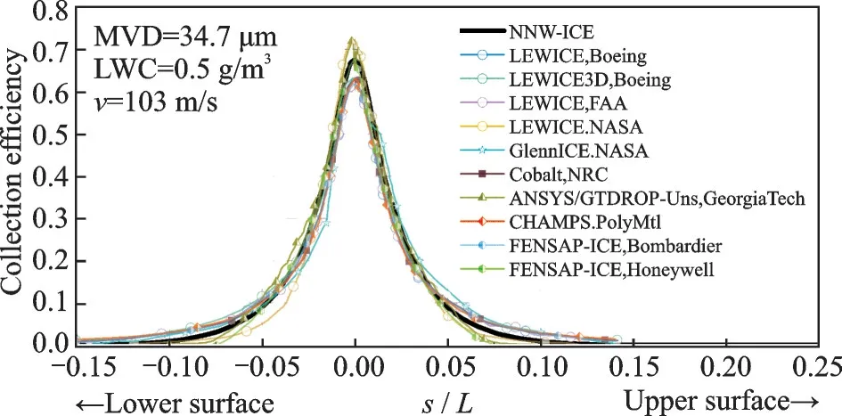
Fig.7 Validation on 3D swept NACA0012 case (IPW 362)

The 3D case of a strait NACA0012 model is compared with various numerical results from the icing prediction workshop （IPW） 2022［27］.The calculation tools and excusive organizations are listed in the graph’s legend.NNW-ICE result is correlated with other results in most part of the curve， and shows slightly higher estimation for peak value.

The validations show that the NNW-ICE droplet solver has equal accuracy to LEWICE and other simulation codes or softwares.

3.2 Validation on BP network with small samples

The BP network is validated by a small number of samples （400）， of which 80% is used for training and the remaining 20% is used for validation.The convergence of error function with iteration is shown in Fig.8.The given spatial coordinate can be diagramed inY-Zcoordinate， while theXcoordinate dimension is considered as priori insignificant.

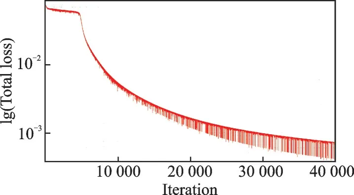
Fig.8 Convergence curve for small samples

Fig.9 shows the predicted probability and error of each validation point.The network correctly predicts all impinged location with at least 90% impinge probability， but makes some incorrect prediction close to the edge of impingement region.The result is considered satisfying because the impingement region is mainly outlined.The error is acceptable to some extent for that the impingement probability will be admissive in a relative low level during actual applications.

3.3 Validation on asynchronous Lagrangian solver

The validation on typical cases will be presented， including a GLC-305 swept airfoil model with root chord length 0.635 m and a nacelle model.The simulation conditions are shown in Table 1.

Table 1 Simulation condition

Validations are made on a X64 windows workstation， with Intel Xeon Gold 6142 CPU， 2.60 GHz.The convergence time is compared for Monte Carlo Lagrangian solver and asynchronous Lagrangian solver.A threads pool with 16 threads in total are used for comparison， of which 10 threads are assigned to BP network， and others are assigned for droplet calculation in asynchronous solver to make balance computing load.In the test for Monte Carlo Lagrangian solver， all 16 threads are used for droplet calculation.

GLC-305 airfoil is meshed with about 1 million hexahedral grids， and the nacelle is meshed with 1.4 million polyhedral grids.The surface meshes are shown in Fig.10.The total droplet number to reach statistical convergence of collection efficiency is 1 million and 4 million， respectively.Each case is divided into 50 time segments.

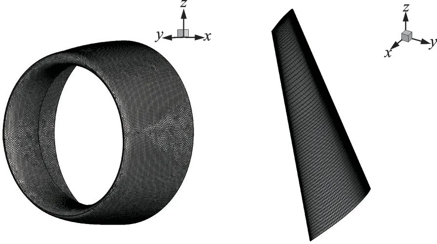
Fig.10 Surface mesh for each validation case

Table 2 shows the convergence time cost for pure Monte Carlo Lagrangian solver and the asynchronous Lagrangian solver accelerated by BP network for validation cases.The asynchronous parallelism saves 26.8% and 24.5% computation time，respectively.It has proven that the Monte Carlo Lagrangian method assisted by BP network is capable to make faster simulation.So far we have reached a satisfying acceleration and it will be hopefully optimized in further study.

Table 2 Time cost comparison for validation cases

3.3.1 GLC-305 swept airfoil case

The calculation result of GLC-305 airfoil is presented in Fig.11.The collection efficiency ofz=0.7 m section is compared in Fig.12.The Monte Carlo Lagrangian solver and asynchronous Lagrangian solver result correlate well， indicating that accuracy is not rejected by the prediction of BP network.

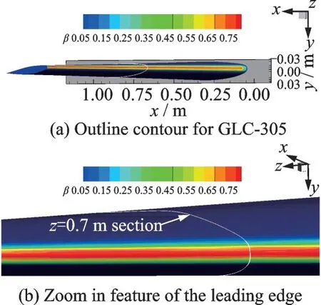
Fig.11 Collection efficiency contour calculation result of GLC-305

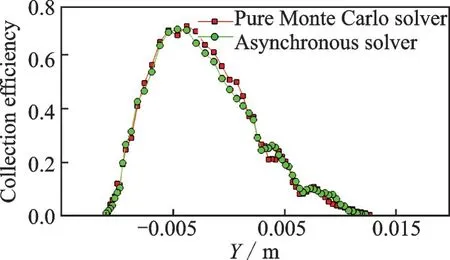
Fig.12 Collection efficiency curve at z=0.7 m section on GLC-305

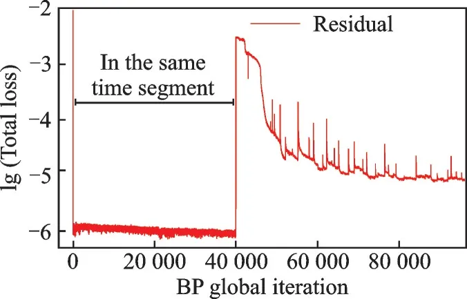
Fig.13 Convergence history by global iterations of BP training for GLC-305 case

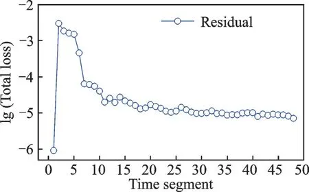
Fig.14 Convergence history by Monte Carlo time segments for GLC-305 case

The convergence curves by time segment and global training iteration are presented in Fig.13 and Fig.14， respectively.The global training iteration refers to the iteration number summed up in each time segment.The error along global training iteration shows a general trend of decreasing， however oscillates when the sample changes.Particularly，the total loss decreases extremely fast to 1E-8 in the first 40 000 iterations， which are all conducted in the same time segment since the samples served in such time segments are in size of hundreds or even fewer， resulting to a fully converged result.However， the BP network trained by such initial samples would not be used for prediction until certain numbers of samples are reached.The total loss is raised as more samples joined in， meanwhile the prediction is adopted to accelerate the droplet solving procedure.This leaves less time for BP network training to reach full convergence.Overall， the total loss decreases despite the oscillation caused by changing samples.

The convergence curve is smoother along time segments， which is considered as time averaged convergence history.The curve indicates that little features are offered by new samples for the BP network since the 10th time segment and afterward.To better improve the asynchronous parallelism， a dynamic assignment of threads is preferred.However，the actual threshold is set to 1E-3 according to previous BP network validation.

3.3.2 Nacelle case

The calculation result of nacelle is presented in Fig.15.A section atz= 0.0 m is sketched with white dot line， at which the collection efficiency is compared for Monte Carlo Lagrangian solve and asynchronous solver results.Fig.16 shows the collection efficiency comparison at sectionz= 0.0 m.

The convergence curve by global training iterations is also presented in Fig.17.The total characteristics for both convergence curves are the same to GLC-305 case.Noted that the oscillations are more vigorous to that of GLC-305 case， and the average value for total loss is around 1E-3 to 1E-4.

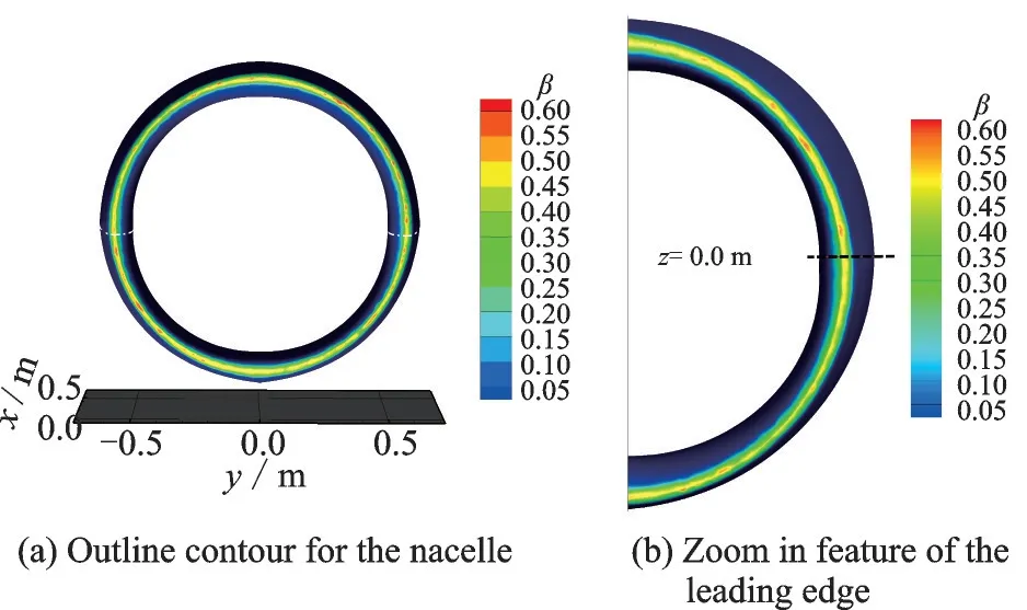
Fig.15 Collection efficiency contour calculation result of nacelle

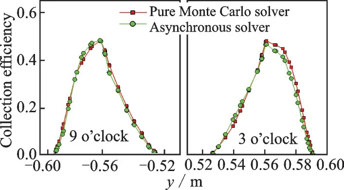
Fig.16 Collection efficiency curve at z = 0.0 m section on nacelle

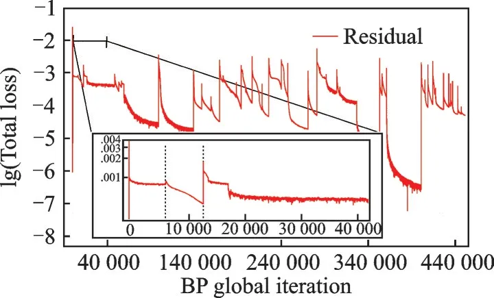
Fig.17 Convergence history by global iterations of BP training for nacelle case

The convergence curve by time segments is presented in Fig.18.The convergence history for nacelle case shows a very unstable training result each time segment and the average total loss is at least one order higher compared to GLC-305 case.It is mentioned that the threshold for BP network convergence is set to 1E-3 in GLC-305， which is also adopted for nacelle case， somehow still valid.The convergence history indicates there is difficulty to make equal prediction for droplet impingement if the geometry complexity increases.

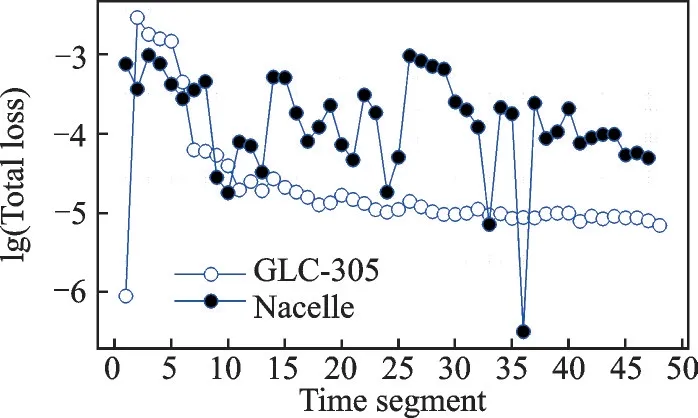
Fig.18 Convergence history by Monte Carlo time segments for nacelle case

An analysis is conducted to reveal the difference for convergence history of GLC-305 case and the nacelle case.The BP network is in fact building a binary classification based on the release positions， which is basically distributed in a 3D plane.The classification on such plane can be depicted as Fig.19 according to priori experience.The topology of impinging area is significantly distinguished.The impinging area for GLC-305 is a typical single connected domain， while the nacelle case is multiplyconnected domain.Thus， the reason could be the simplicity of BP network.The features of sample data are not fully decomposed by limited neurons in such binary classification problem.

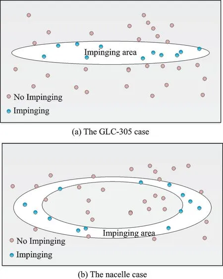
Fig.19 Topology for impinging area on releasing plane

4 Conclusions

The work of this study can be concluded as follows：

（1） An asynchronous parallelism is applied on NNW-ICE software to merge the Monte Carlo Lagrangian droplet solver and the BP neural network as a synchronous solver for droplets.The Monte Carlo method is applied to obtain statistical mass flow rate and collection efficiency at the target surface.The backpropagation neural network is introduced to provide a quick prediction for droplet impingement probability.The BP network is constructed with a 3×4×4×2×1 structure， with the ELU function for hidden layers and the sigmoid function for the output layer.The momentum BP method and variable learning rate technique are employed to achieve better convergence.To make the BP network universally applicable， an asynchronous Lagrangian solver is developed， in which the Monte Carlo Lagrangian solver and the BP network training are paralleled un-interfere， but only communicate at two synchronize points.

（2） A 3D GLC-305 airfoil model and a jet-engine nacelle model are used to validate the asynchronous solver.The result shows significant acceleration for both cases， while the accuracy is not affected by the BP network prediction.This study represents the first attempt to deeply integrate the artificial neural network with aircraft icing simulation method.The neural network technique shows a great potential in resolving the disadvantages of Lagrangian method.

（3） The presented study will be developed in the upcoming works， with further optimization of the ANN architecture and the development of an adaptive strategy for Monte Carlo method based on network prediction.