Underwater acoustic signal denoising model based on secondary variational mode decomposition
Hong Yang, Wen-shuai Shi, Guo-hui Li
School of Electronic Engineering, Xi'an University of Posts and Telecommunications, Xi'an, Shaanxi, 710121, China
Keywords:Underwater acoustic signal Denoising Variational mode decomposition Secondary decomposition Fluctuation-based dispersion entropy Cosine similarity
ABSTRACT Due to the complexity of marine environment, underwater acoustic signal will be affected by complex background noise during transmission.Underwater acoustic signal denoising is always a difficult problem in underwater acoustic signal processing.To obtain a better denoising effect, a new denoising method of underwater acoustic signal based on optimized variational mode decomposition by black widow optimization algorithm (BVMD), fluctuation-based dispersion entropy threshold improved by Otsu method (OFDE), cosine similarity stationary threshold (CSST), BVMD, fluctuation-based dispersion entropy (FDE), named BVMD-OFDE-CSST-BVMD-FDE, is proposed.In the first place, decompose the original signal into a series of intrinsic mode functions (IMFs) by BVMD.Afterwards, distinguish pure IMFs,mixed IMFs and noise IMFs by OFDE and CSST,and reconstruct pure IMFs and mixed IMFs to obtain primary denoised signal.In the end, decompose primary denoising signal into IMFs by BVMD again,use the FDE value to distinguish noise IMFs and pure IMFs, and reconstruct pure IMFs to obtain the final denoised signal.The proposed mothod has three advantages: (i) BVMD can adaptively select the decomposition layer and penalty factor of VMD.(ii)FDE and CS are used as double criteria to distinguish noise IMFs from useful IMFs, and Otsu algorithm and CSST algorithm can effectively avoid the error caused by manually selecting thresholds.(iii)Secondary decomposition can make up for the deficiency of primary decomposition and further remove a small amount of noise.The chaotic signal and real ship signal are denoised.The experiment result shows that the proposed method can effectively denoise.It improves the denoising effect after primary decomposition, and has good practical value.
1.Introduction
1.1.Research background
Underwater acoustic signal denoising is the foundation of underwater acoustic signal processing.The existence of noise will seriously affect the subsequent processing effect [1].Underwater acoustic signal is not only non-Gaussian, nonlinear and nonstationary [2,3], but also chaotic [4].Underwater acoustic signal is often interfered by the noise of the ocean environment during transmission, which leads to the distortion of the waveform of underwater acoustic signal.Due to the progress of concealment technology of modern marine ships, underwater acoustic signal that can be detected is getting weaker and weaker, and it is more and more difficult to reduce the noise in underwater acoustic signal[5].This brings severe challenges to the research of underwater target location and tracking, and the detection and recognition of underwater acoustic signal [6,7].Therefore, we urgently seek an effective denoising method for underwater acoustic signal.
1.2.Literature review
In recent years, people have proposed various denoising methods for underwater acoustic signal.It can be divided into two categories: traditional denoising method and decomposition and integration denoising method.
(1) Traditional denoising method of underwater acoustic signal include local projection algorithm (LP) [8,9], wavelet transform (WT) [10], compressed sensing method (CS) [11,12],blind source separation (BSS) [13], principal component analysis (PCA) [14], independent component analysis(ICA)[15],sparse decomposition(SD)[16],etc.These methods have a certain denoising effect, but the denoising effect of nonlinear underwater acoustic signal can't reach a satisfactory level.
(2) Empirical mode decomposition (EMD) is a time frequency domain processing method to analyze nonlinear and nonstationary signal [17-19].Due to EMD has the mode mixing problem, some improved algorithms such as ensemble EMD (EEMD), complementary ensemble EMD (CEEMD),complete EEMD with adaptive noise (CEEMDAN) and variational mode decomposition (VMD) are proposed [20-23].Some scholars use different mode decomposition algorithms to decompose signal into a series of intrinsic mode functions(IMFs).Apply different criterias such as sample entropy(SampEn) [24], permutation entropy (PE) [25], Pearson correlation coefficient [26], mutual information [27,28], etc,selecte the useful components to achieve the purpose of denoising.At present, decomposition and integration denoising method mainly has the following two ideas.An idea is to remove useless components and reconstruct useful components according to criterias, such as EMD-MPE [29],CEEMDAN-FE[30],IVMD-SE[31],VMD-MPE[32],VMD-NPE[33], UPEMD-AAPE-PCC [34], CEEMDAN-ED-EE [35], IVMDMIC-PE [36], ICEEMDAN-norMI-MIPE [37].The other idea is to classify the mode components according to the decision criteria, adopt different denoising method according to the categories, and finally reconstruct the signal, such as CEEMDAN-MI-PE-WT[38],MCEEMDAN-DE-IT[39],MIVMDMDE-LWTD-SG [40], SVMD-SdrSampEn-IWTD-SG [41],CEEMDAN-MMSVC-LMSAF[42],CEEMDAN-ETC-RCMDE-WT[43].
These methods can suppress noise to a certain extent,but there are still some limitations: (i) Decomposition layer and the penalty factor of VMD are not well set.(ii) Entropy, correlation coefficient,mutual information and other thresholds that can distinguish useful components need to be set manually.(iii) Inadequate decomposition will lose some useful information.Details of these methods mentioned in this section are shown in Table 1.
1.3.Aims and innovations
To obtain a better denoising effect, a new denoising method of underwater acoustic signal based on optimized variational mode decomposition by black widow optimization algorithm (BVMD),fluctuation-based dispersion entropy threshold improved by Otsu method (OFDE), cosine similarity stationary threshold (CSST),BVMD,fluctuation-based dispersion entropy (FDE),named BVMDOFDE-CSST-BVMD-FDE,is proposed.The main innovations are
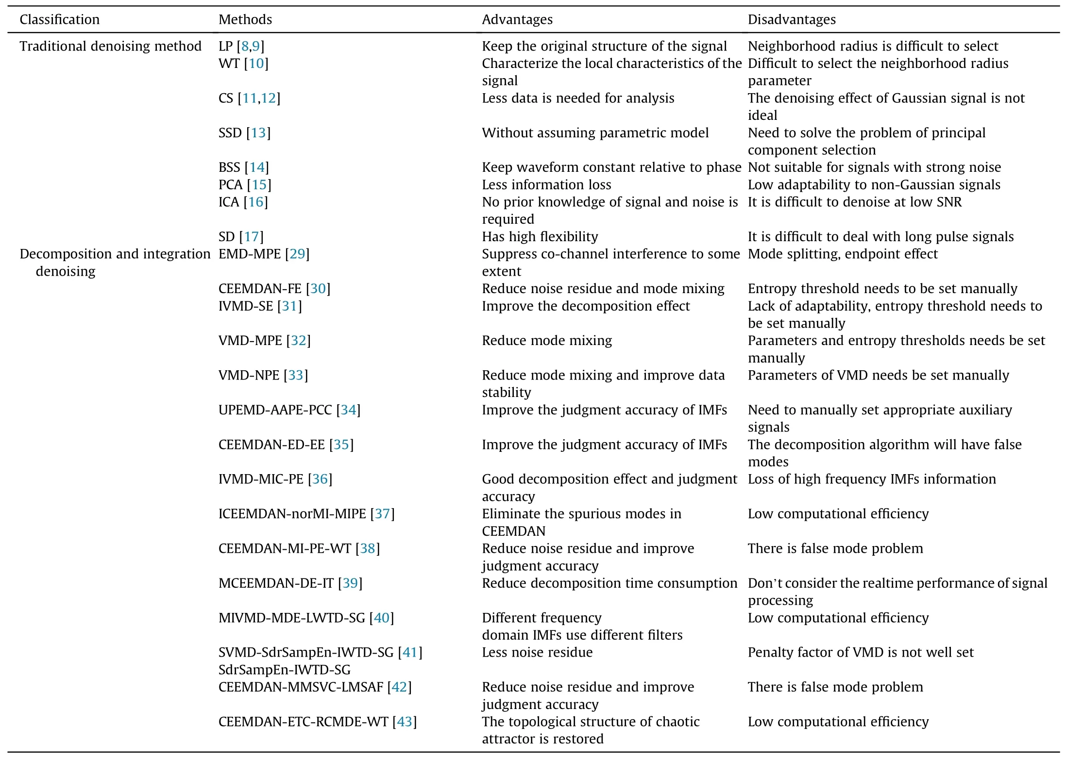
Table 1Detail of the methods mentioned in the introduction.
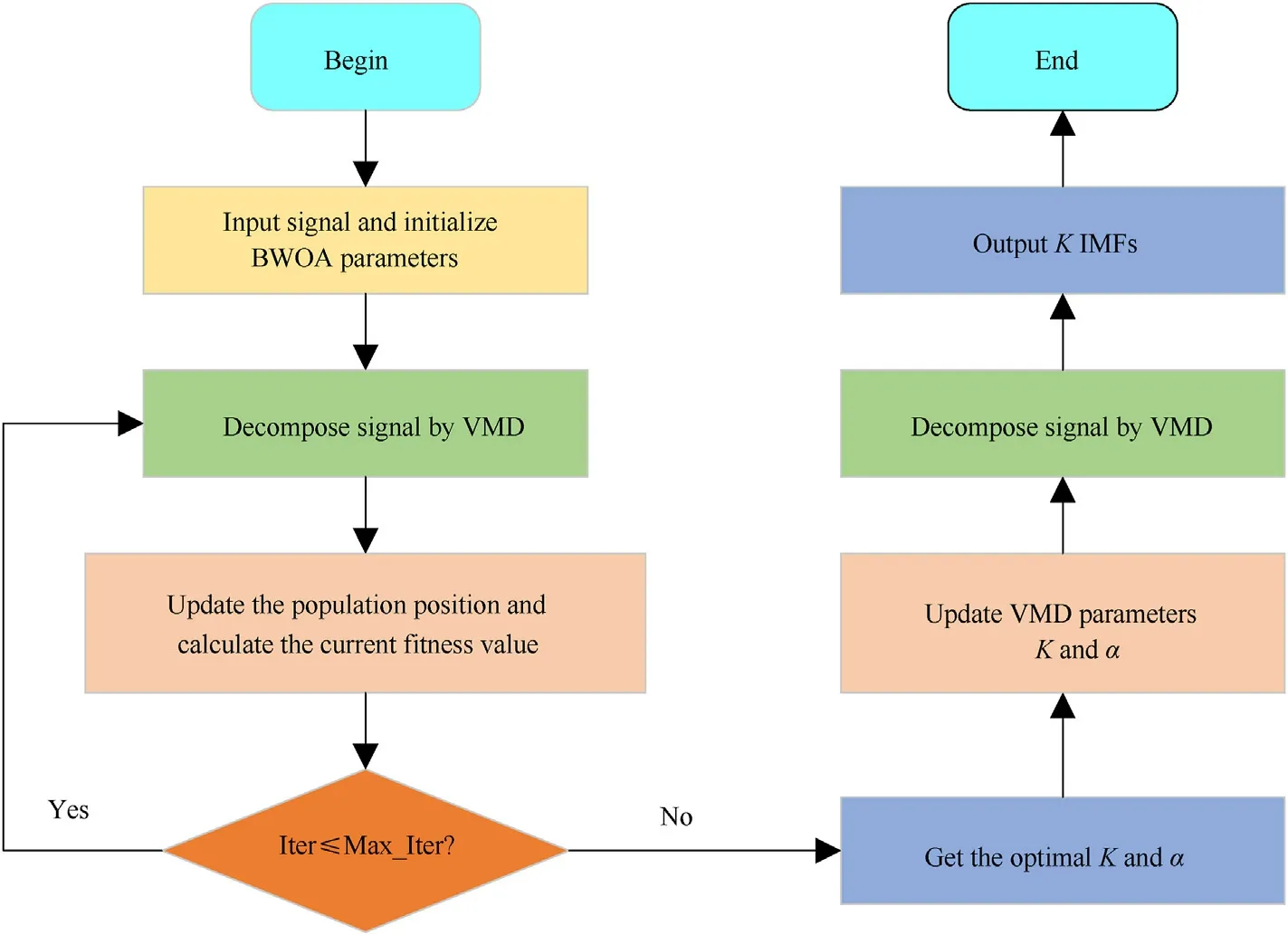
Fig.1.The specific process of BVMD.
(1) Optimized variational mode decomposition by black widow optimization algorithm, named BVMD, is proposed.It can adaptively select decomposition layer and penalty factor of VMD.
(2) Fluctuation-based dispersion entropy threshold improved by Otsu method, named OFDE, is proposed.Cosine similarity stationary threshold, named CSST, is proposed.OFDE and CSST can effectively avoid the error caused by manually selecting threshold.
(3) Secondary decomposition can make up for the deficiency of primary decomposition and further remove noise.
The structure of this paper is as follows:The second part is basic theory.The third part is the proposed method and evaluation standard.The fourth part is experiment and analysis.The fifth part is discussion.The sixth part is conclusions.
2.Basic theory
2.1.Optimized variational mode decomposition by black widow optimization algorithm
2.1.1.Variational mode decomposition
Variational mode decomposition (VMD) is an adaptive time frequency domain processing method to signal[44].It is considered that the signal is composed of K IMFs with limited bandwidth,and each IMF has its own center frequency and bandwidth.The specific steps are [45]
Step 1:Analyze the K mode functions by Hilbert transform to get the unilateral spectrum of the signal mode
Step 2: Multiply the exponential term e-jwktof the central frequency wkwith the frequency spectrum, and modulate the central band of the signal to the corresponding baseband
Step 3: Calculate the square sum of the L2norm of the time domain gradient of Eq.(2) and estimate the sum of all bandwidths.The variational problem of its constraint conditions is as follows:
where Luk(t)represents the corresponding K IMFs,min represents the minimum constraint, wk(t) represents the center frequency of the K IMFs respectively, j represents imaginary number, δ(t) represents the unit impact function, * represents convolution calculation.
Step 4: Introduce penalty factor α and augmented Lagrange multiplier λ into the above variational constraint model, and transform the constrained variational problem into an unconstrained variational problem

where ε is the judgment precision.
2.1.2.Black widow optimization algorithm
Black widow optimization algorithm (BWOA) mainly simulates the life cycle of the black widow spider [46].BWOA has the characteristics of fast convergence and high accuracy.BWOA includes five stages: initialization population, reproduction, cannibalism,mutation and update population.The specific steps are [47]
Step 1: Initialize population
In BWOA,each solution of the problem to be solved is regarded as each black widow spider,and each black widow spider is merged into a one-dimensional array
where N is the dimension of array features.Each feature value at initialization is a random floating-point number.Each black widow spider has its fitness.Usually, an array is brought into a fitness function to calculate the fitness
Initializing population requires predefining Npopblack widow spiders in advance to obtain a Npop×N generating matrix

Fig.2.The specific process of OFDE.
where Npopcan be defined as 30 or 50 in advance as required.
Step 2: Reproduction
The reproductive stage is the global search stage.According to the value of Fitness,the population of black widow spiders is sorted,and the number of black widow spiders participating in reproduction is calculated according to the procreating rate criterion.According to the random criterion,a pair of black widow spiders are selected to reproduce.In the process of reproduction,it is separated from other black widow spiders and does not interfere with each other.Each reproduction produces about 1000 eggs,and only those with strong vitality can survive.In the black widow algorithm,each parent simulates the reproductive process with the help of α array

Fig.3.The flow chart of the proposed method.

Table 2The values of SampEn, FDE and PE.
where W1and W2are parents,child1and child2are offspring.This process has to be repeated N/2 times.
Step 3: Cannibalism
Cannibalism refers to spiders with high adaptability eat spiders with low adaptability.The cannibalism of the widow spider can be divided into three types: sexual cannibalism, sibling cannibalism and female cannibalism.Sexual cannibalism refers to that the female black widow will eat the male black widow during or after mating.Sibling cannibalism refers to about a week after the young spider hatches, brothers and sisters cannibalize.Female cannibalism refers to the event that a small spider eats a female spider.In the black widow algorithm, sexual cannibalism and sibling cannibalism are simulated.By destroying the father to achievecannibalism, and destroying some children according to cannibalism rate, brothers and sisters can achieve cannibalism.The fitness value is used to determine the strength of young spiders.

Table 3The values of SampEn, FDE and PE.

Fig.4.The change of SampEn, FDE and PE with different SNR.
Step 4: Mutation
The mutation stage is the local search stage.At this stage, the black widow algorithm randomly selects several black widows according to mutation rate, and each black widow randomly exchanges two eigenvalues in the array.
Step 5: Update population
After the first iteration, the black widows retained in the cannibalism phase and mutation phase are taken as the initial population of the next iteration:
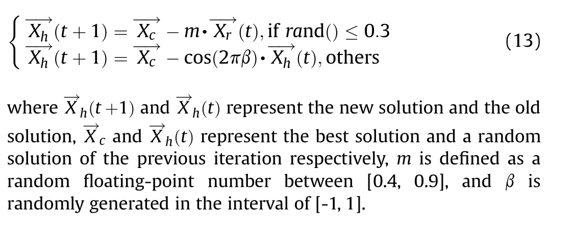
Step 6: Stop condition
Stop condition can be considered:(1)Set the maximum number of iterations.(2) The position of the best black widow no longer changes.(3) Achieve the preset accuracy.
2.1.3.BVMD
VMD has the characteristics of adaptive decomposition.However, when using VMD to decompose the original data, decomposition layer K and penalty factor α should be set in advance.The setting of K and α will directly affect the decomposition effect,but the decomposition effect by manually setting parameters is often inaccurate.BWOA has the characteristics of fast optimization speed and high precision.To determine the optimal combination of K and α, optimized variational mode decomposition by black widow optimization algorithm, named BVMD, is proposed.
Select SampEn as the fitness function of BWOA.For N-dimensional time series: ˙Xt= {˙x(1), ˙x(2),., ˙x(N)}, SampEn is defined as

Fig.1 shows the specific process of BVMD.The specific steps are
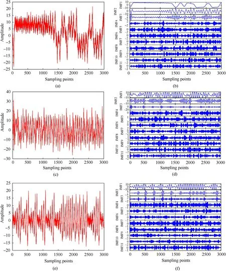
Fig.5.The time domain diagrams and the decomposition results of BVMD: (a) and (b) Lorenz, (c) and (d) Chen, (e) and (f) Rossler.

Table 4The results of FDE values.
Step 1: Initialize BWOA parameters, and set the population number to 50, the number of iterations to 10,the range of K to Refs.[3,11], and the range of α to [1000,4000].
Step 2: Decompose signal by VMD.
Step 3: Calculate SampEn by Eq.(14) to get the fitness.
Step 5: Repeat steps 2, 3 and 4, until reach the maximum number of iterations.
Step 6: Get the optimal parameter pair (K,α) of VMD.
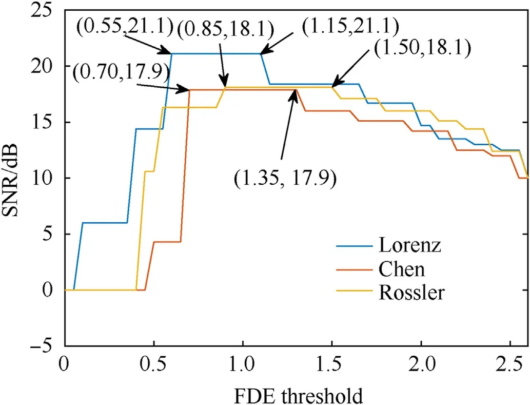
Fig.6.The change of SNR of different signals with threshold values.
Step 7: Update VMD parameters K and α.
Step 8: Decompose signal by VMD.
Step 9: Output K IMFs.
2.2.Fluctuation-based dispersion entropy threshold improved by Otsu method
2.2.1.Otsu method
Otsu method is an efficient algorithm for image binarization.It is the optimal segmentation in the sense of least square method.The specific steps are [48]:
So they were drowned, repeated Anne Lisbeth; but she said nomore, and the subject was dropped. She felt very low-spirited, because her count-child had shown no inclination to speak to her who loved him so well, and who had travelled so far to see him. The journey had cost money too, and she had derived no great pleasure from it. Still she said not a word of all this; she could not relieve her heart by telling the laborer s wife, lest the latter should think she did not enjoy her former position at the castle. Then the raven flew over her, screaming again as he flew.
Step 1: Assume that the gray scale is divided into L levels, the total number of all pixels is N,and set the number of pixels in the i-th gray scale is ni, then all the pixels in the image are
Step 2:Set Pito represent the probability distribution of pixels in the i-th gray level
Step 3: Set a gray level threshold K in advance, the gray levels can be divided into two categories base on the threshold,which are the target image C0and the background C1.C0is consists of pixels with gray values between[1,K],and C1is consists of pixels with gray values between [K +1,L - 1].The distribution probability of C0and C1is
Step 4:Average and global average of these two types of C0and C1can be expressed as
where u0is the average gray value of C0,u1is the average gray value of C1,and uTrepresents the average gray value of the whole picture.Step 5:The variance between classes between the target image and the background is

2.2.2.Fluctuation-based dispersion entropy
FDE is a nonlinear dynamic analysis method to describe the complexity and irregularity of time series.It is very sensitive to noise.The more noise the signal contains, the greater the complexity and irregularity of the time series of the signal and thegreater the FDE value [49,50].Its steps are

Table 5The CS value of each IMF after three kinds of noisy signals are decomposed by BVMD.
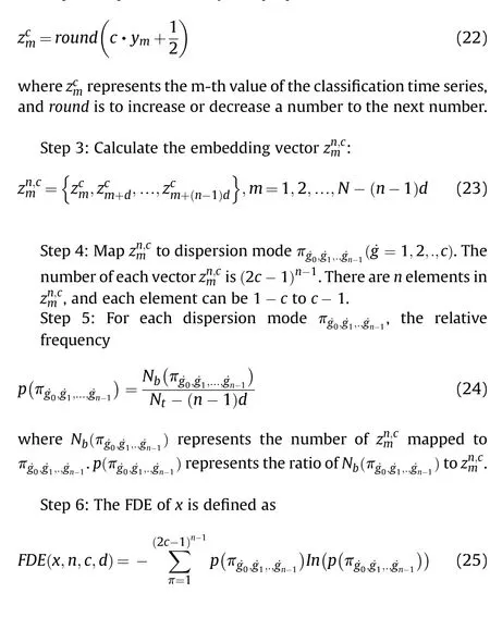
Step 1: Time series x = {xm,m = 1,2,.,Nt}, and map x to y={ym,m=1,2,.,Nt} according to the normal distribution function
where μ and σ respectively represent the expected value and standard deviation of time series.
Step 2: Map the value of ymto[1,c]
2.2.3.Fluctuation-based dispersion entropy threshold improved by Otsu method
In this section, fluctuation-based dispersion entropy threshold improved by Otsu method, named OFDE, is proposed.The basic principle of Otsu method is to calculate the variance between two kinds of backgrounds according to the gray threshold.When the variance reaches the maximum,it means that the error probability is the smallest, and the segmentation edge between the target object and the background can be well found according to its threshold.
In view of the accuracy and stability of FDE in calculating the complexity of time series.Therefore, the complexity of time series can be transformed into the relationship between FDE values.Use Otsu method to calculate the variance between signals according to the entropy threshold.When the variance reaches the maximum,the corresponding FDE value is the threshold for distinguishing signals.Fig.2 shows the specific process of OFDE.The specific steps are
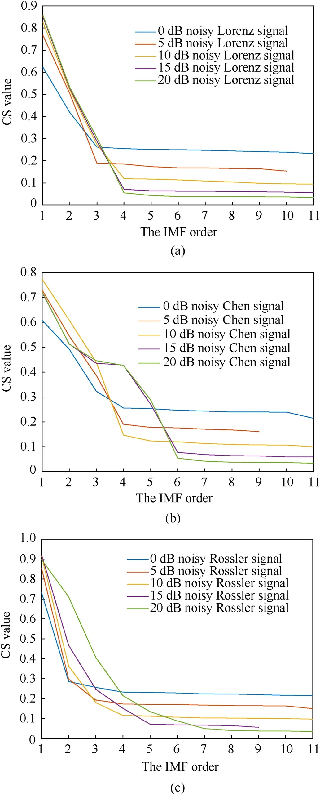
Fig.7.The CS change curves: (a) Lorenz; (b) Chen; (c) Rossler.

Table 6The CSST values of three kinds of noisy signals.
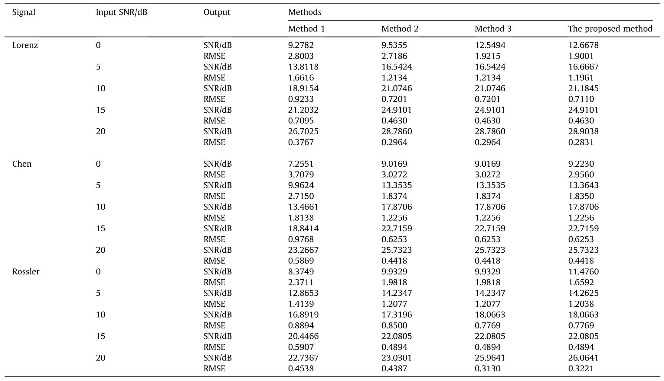
Table 7The denoising results.
Step 1:Decompose the signal into IMFs by BVMD,and calculate the FDE value of each IMF
Step 2:Sort the FDE values and define the probability Pi=1/N of each entropy FDEi.The average and global average of the low complexity sequence C0and the high complexity sequence C1can be expressed as
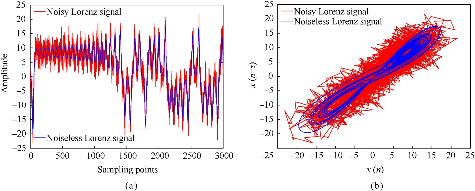
Fig.8.The time domain diagram and the phase diagram: (a) and (b) noisy and noiseless Lorenz signal.
where ω0represents the probability of low complexity sequence C0,ω1represents the probability of high complexity sequence C1, u0represents the average entropy of C0, u1represents the average entropy of C1, and uTrepresents the global entropy.Step 3: Set the initial threshold K = min FDEi, and set the step h = 1.Calculate the variance between classes σ2Kevery time until K = max FDEi.The variance between classes is:

2.3.Cosine similarity stationary threshold
2.3.1.Cosine similarity
Cosine similarity (CS) can be used to measure the difference between two vectors in space.The range of CS is[-1,1].The closer the CS value is to 1,the more similar the two vectors are.The angle between vectors x and y is called θ [51].Cosine value is
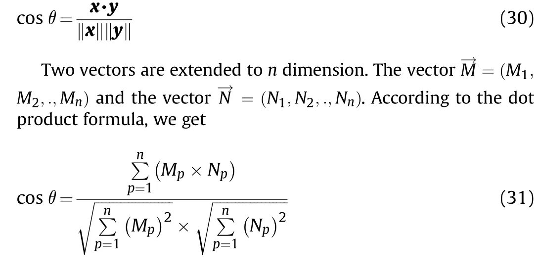
2.3.2.Cosine similarity stationary threshold
In this section, cosine similarity stationary threshold (CSST) is proposed.According to CSST, signals with high similarity can be found, which avoids the error caused by using fixed threshold.Its principle is:
When the similarity reaches a steady state,its signal is judged as a low similarity signal.Set the sum of the absolute values of CS change of three consecutive signals to be less than a certain value as the judgment condition
where CSirepresents the similarity value of the i-th signal, φ represents the stationary condition, and set φ=0.02 in this section.When the first CSST meets the conditions,the CS value of the first signal is the threshold.The specific steps are as follows:
Step 1:Decompose the original signal into K IMFs by BVMD,and calculate the CS value.
Step 2: Sort the CS values from big to small, calculate CSSTi=|CSi-CSi+1|+|CSi+1-CSi+2|.When the first CSST is less than φ,corresponding CSiis the required threshold.
3.The proposed method and evaluation standard
3.1.The proposed method
To obtain a better denoising effect, a new denoising method of underwater acoustic signal based on optimized variational mode decomposition by black widow optimization algorithm (BVMD),fluctuation-based dispersion entropy threshold improved by Otsu method (OFDE), cosine similarity stationary threshold (CSST),BVMD,fluctuation-based dispersion entropy (FDE),named BVMDOFDE-CSST-BVMD-FDE,is proposed.The flow chart of the proposed method is shown in Fig.3.The specific steps are
Step 1: Decompose the original signal into IMFs by BVMD.
Step 2: Calculate the FDE value and CS value of each IMF.
Step 3: Set the entropy threshold θ by OFDE, and the similarity threshold σ by CSST.
Step 4:Consider IMFs as pure IMFs if the FDE value of IMFs is less than θ and greater than σ.Considered IMFs as noise IMFs if the FDE value of IMFs is greater than θ and less than σ.Consider the remaining IMFs as mixed IMFs.Reconstruct pure IMFs and mixed IMFs to obtain primary denoised signal.

Fig.9.(a) The result of BVMD; (b) The frequency domain diagram; (c) The variation curve of fitness value.
Step 5.Decompose primary denoised signal into IMFs by BVMD again.
Step 6.Calculate the FDE value of each IMF after decomposition,and remove the IMFs larger than threshold η to obtain the final denoised signal.
3.2.Evaluation standard
3.2.1.Evaluation standard of chaotic signal denoising
Selecte signal to noise ratio (SNR) and root mean square error(RMSE) as evaluation criteria of chaotic signal denoising in this paper.
where x︵(p) represents the original signal, ~x(p) represents a denoised signal, and P represents the number of sampling sequences of the signal.The larger the SNR,the smaller the RMSE,and the better the denoising effect.
3.2.2.Evaluation standard of underwater acoustic signal denoising
Selecte correlation dimension (CD), noise intensity (NI) [52],attractor phase diagram and FDE to evaluate the denoising effect of underwater acoustic signal.
(1) NI

Fig.10.(a) The result of EMD, (b) the frequency domain diagram.

Table 8The FDE value and CS value.

(2) CD
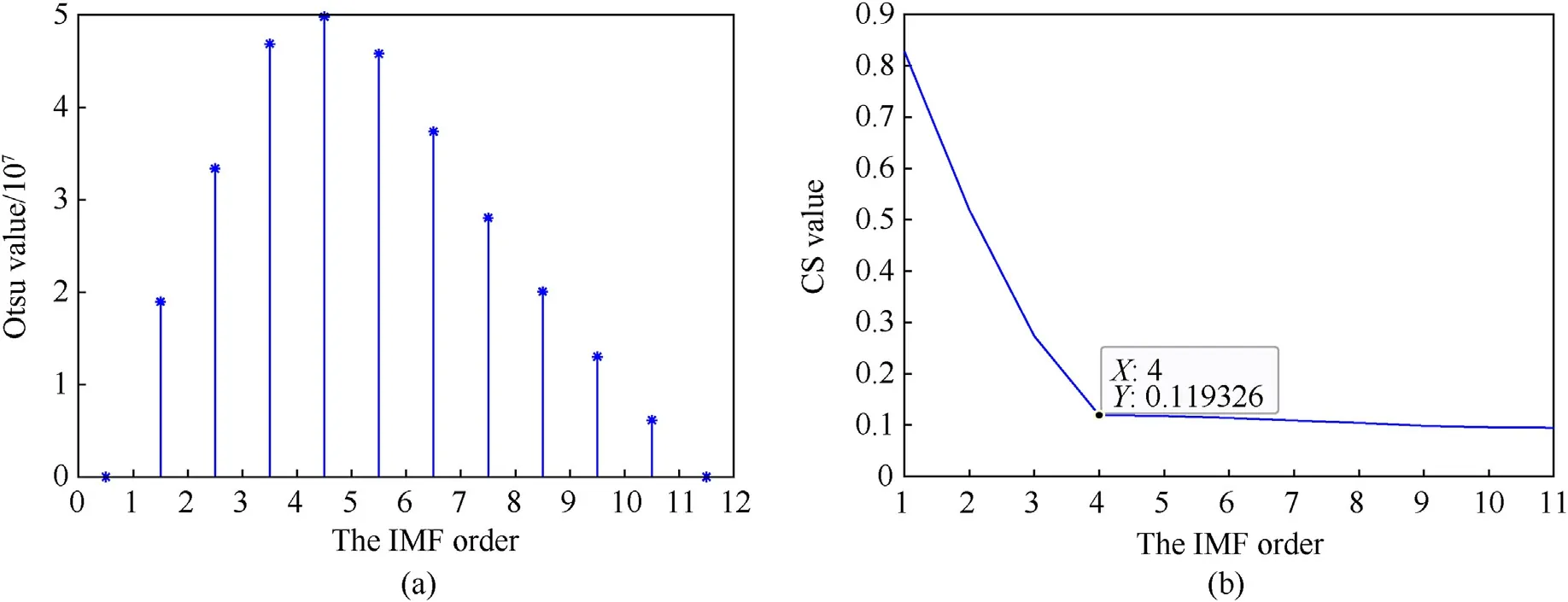
Fig.11.The change of value: (a) Otsu; (b) CS.

Table 9The FDE value of each IMF after secondary decomposition by BVMD.
The calculation of attractor dimension plays an important role in chaos analysis, and CD is an important parameter to describe attractor dimension[53].The calculation and analysis of CD can be applied to describe the change of chaotic system.The correlation dimension method is used to describe the chaotic characteristics of signals.Set the embedding dimension to l and the delay time to ˙τ.The phase space of time sequence {x1,x2,.,xk} is
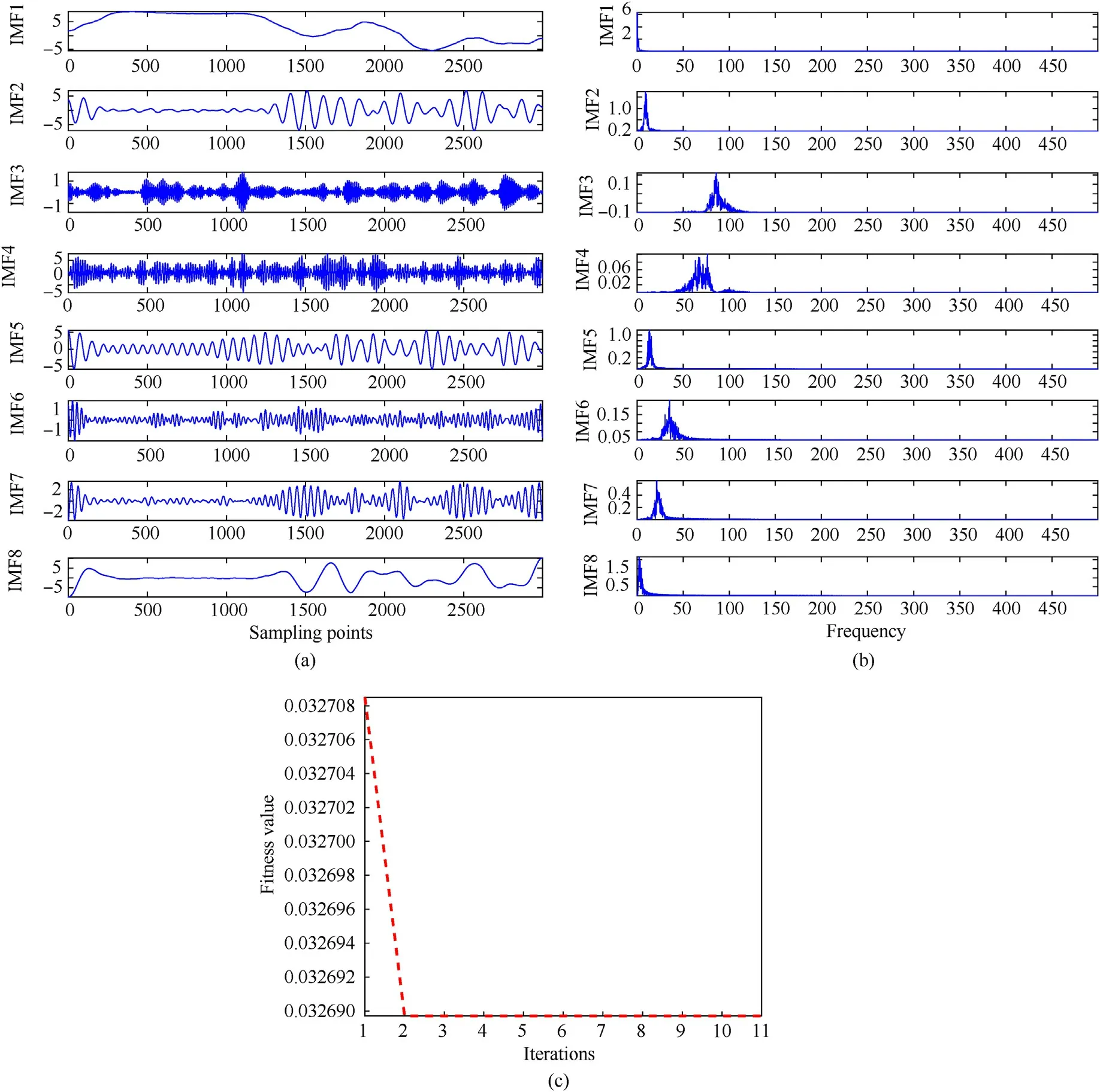
Fig.12.(a) The secondary decomposition result of BVMD; (b) The frequency domain diagram; (c) The variation curve of fitness value.
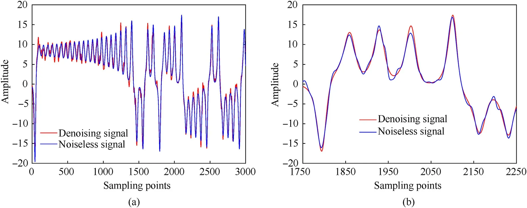
Fig.13.Before and after denoising by method 1: (a) The time domain diagram; (b) Local detail diagram.
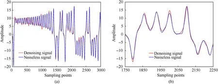
Fig.14.Before and after denoising by method 1 and 3: (a) The time domain diagram; (b) Local detail diagram.
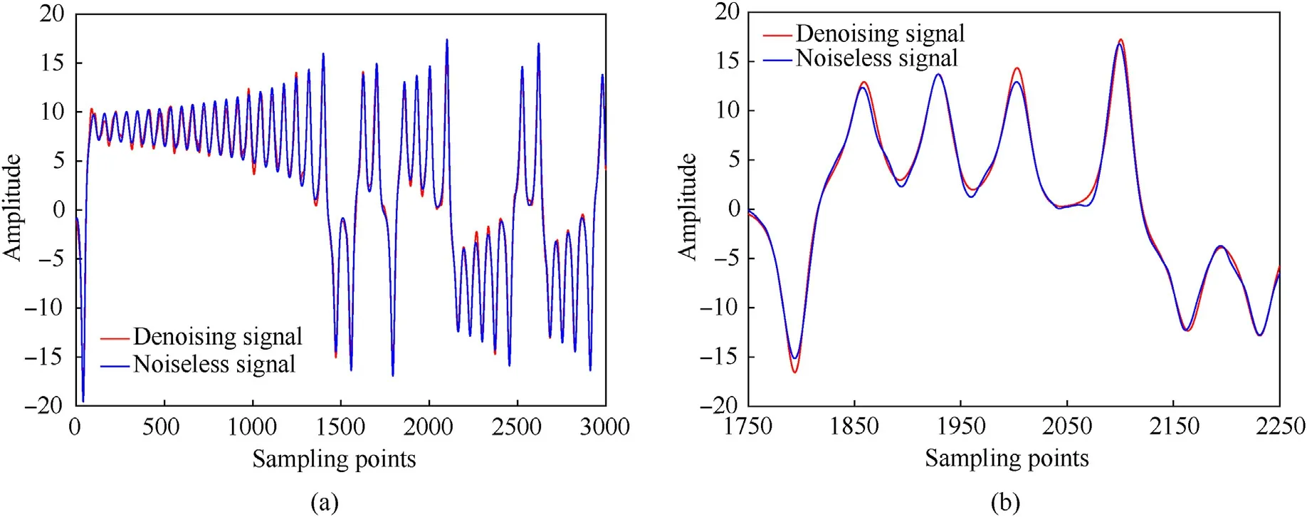
Fig.15.Before and after denoising by the proposed method: (a) The time domain diagram; (b) Local detail diagram.
where Nxis Nxvectors in the reconstructed space.
The one-dimensional sequence is embedded into multidimensional space,which is transformed into a set of vectors:ym= [xm,xm+˙τ,xm+2˙τ,.,xm+(l-1)˙τ].The distance between any two vectors ymand ynis
Get the correlation integral function
where r>0, J(x) is a step function
Let dmaxbe the maximum extension distance of the attractor in m-dimensional space.The correlation integral function can be expressed as
The correlation dimension D is obtained
(3) Attractor phase diagram
In nonlinear dynamical system, attractor is an important property to determine the state space.Chaos is a nonlinear phenomenon, and the most classical method of observing chaotic system is phase diagram.The smoother the curve of the phase diagram, the stronger the regularity,indicating that the noise of the signal in the chaotic system is less [54].
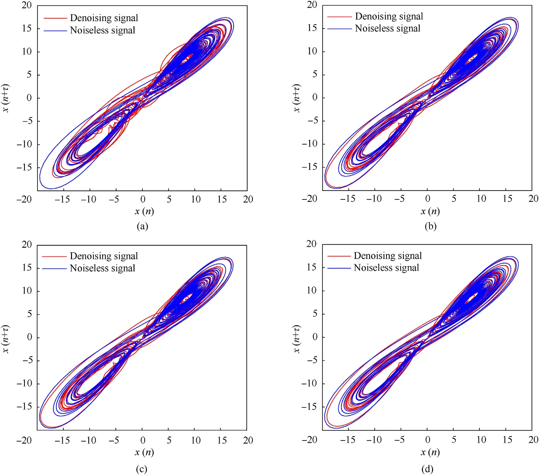
Fig.16.The denoised phase diagrams: (a) Methods 1; (b) mMethods 2; (c) Methods 3; (d) The proposed method.

Table 10Four types of ship signals used in the experiment.
4.Experiment and analysis
In a real underwater environment, noise is not caused by a single sound source, it often consists of noise from many different sources[55].Most underwater acoustic signal processing methods are based on the assumption of Gaussian noise[56].In Refs.[38,57],the authors also added different decibels of white Gaussian noise in his underwater acoustic signal simulation experiment.Liu et al.have shown that short-term marine environmental noise follows Gaussian distribution[58].First of all,the simulation data selected in our experiment is to intercept a very small part of the signals for experimental analysis, which meets the requirement of obeying Gaussian distribution in a short time.Secondly, when the noise source of real noise is unclear, white Gaussian noise is the best simulation of real noise.Finally,adding white Gaussian noise in the simulation experiment is convenient for quantification and experimental analysis, and the quality of denoising methods can be objectively observed.Based on the above description,we add white Gaussian noise with different SNR in the simulation experiment to do the denoising experiment analysis.Select three typical chaotic signals such as Lorenz signal, Chen signal and Rossler signal for simulation experiment as pure signal.Use EMD-FDE, BVMD-FDE and BVMD-OFDE-CSST as comparison methods.Section 4.1 is performance analysis of FDE.Section 4.2 is FDE threshold selection experiment.Section 4.3 is CS threshold selection experiment.Section 4.4 is chaotic signal denoising experiment.Section 4.5 is underwater acoustic signal denoising experiment.
4.1.Performance analysis of FDE
Design the follow experiments to verify the superiority of FDE.Add 10 dB white Gaussian noise to the simulation signal cos(2πft)with signal frequencies of 20 Hz, 50 Hz and 100 Hz, and calculate the values of SampEn, FDE and PE respectively.Table 2 shows the results.

Fig.17.The time domain diagram and phase diagram of four kinds of ship signals before denoising: (a) and (b) S-1; (c) and (d) S-2; (e) and (f) S-3; (g) and (h) S-4.

Table 11CS and FDE values.
Add white noise signal from 0 to 19 dB to the simulation signal cos(2πft)with a signal frequency of 100 Hz.Calculate the values of SampEn, FDE and PE respectively.Table 3 shows the calculation results.The result change after the entropy value is normalized is shown in Fig.4.
As shown in Table 2, compared with the other two kinds of entropy,the calculation result of FDE is more accurate;the change range of PE is small,it is difficult to detect the signal change,and the effect is the worst.As shown in Fig.4, FDE is more stable than SampEn and PE,and can accurately measure the complexity of time series.
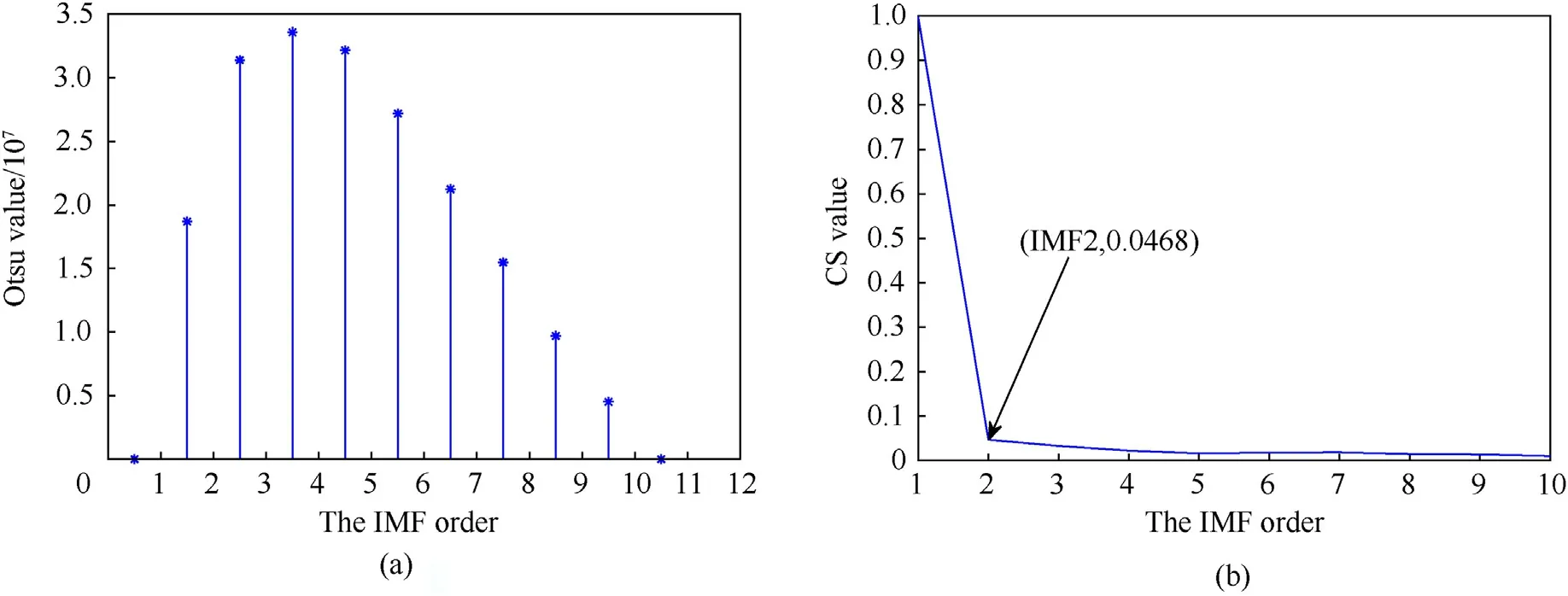
Fig.19.The change of value: (a) Otsu; (b) CS.

Table 12The FDE values of each IMF after secondary decomposition.
4.2.FDE threshold selection experiment
To select a appropriate threshold of FDE to distinguish the useful IMFs of BVMD-FDE method, the following experiment will be conducted.Lorenz system, Chen system and Rossler system are follows:
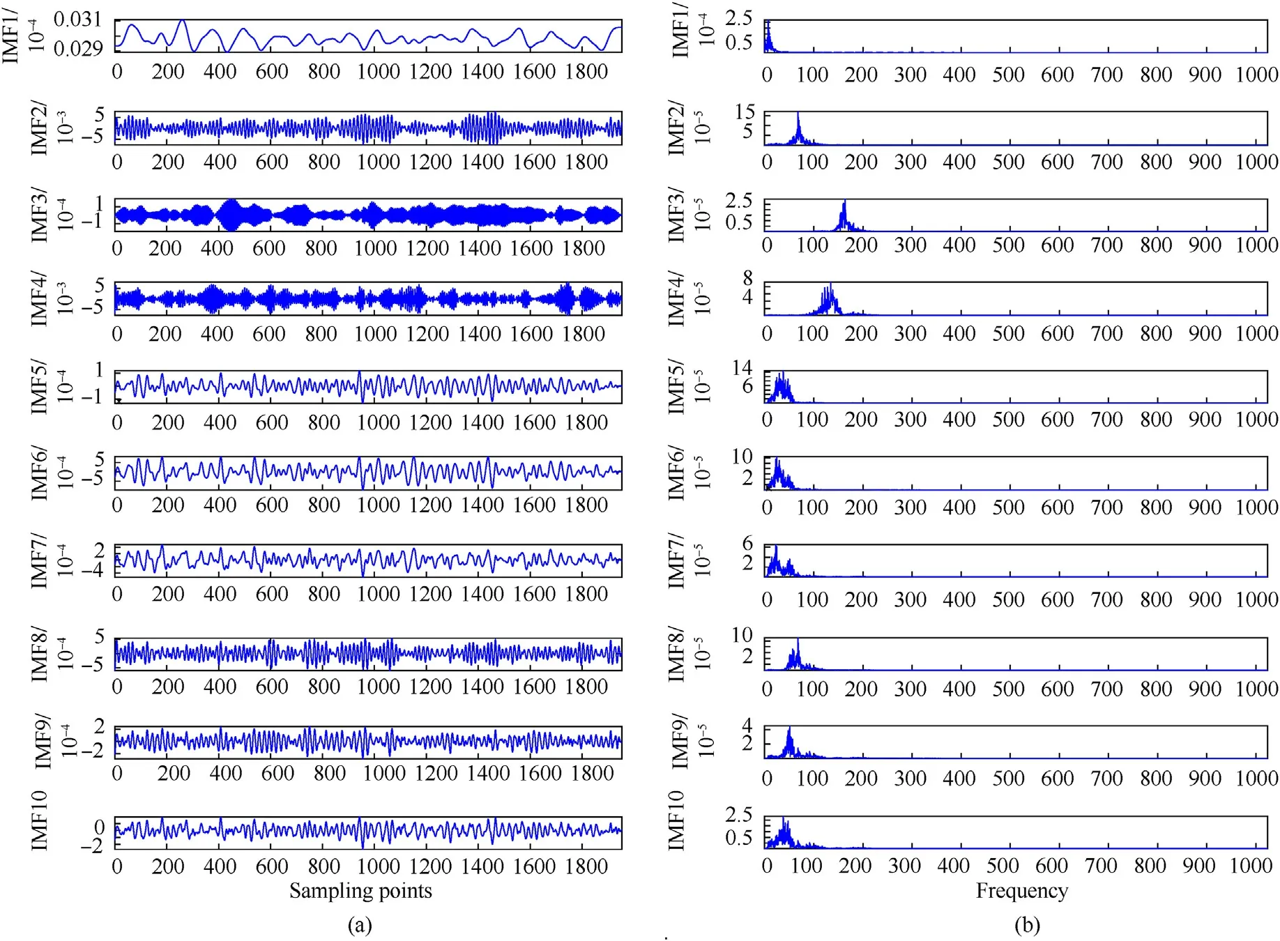
Fig.20.(a) The results of secondary decomposition by BVMD; (b) Frequency domain diagram.
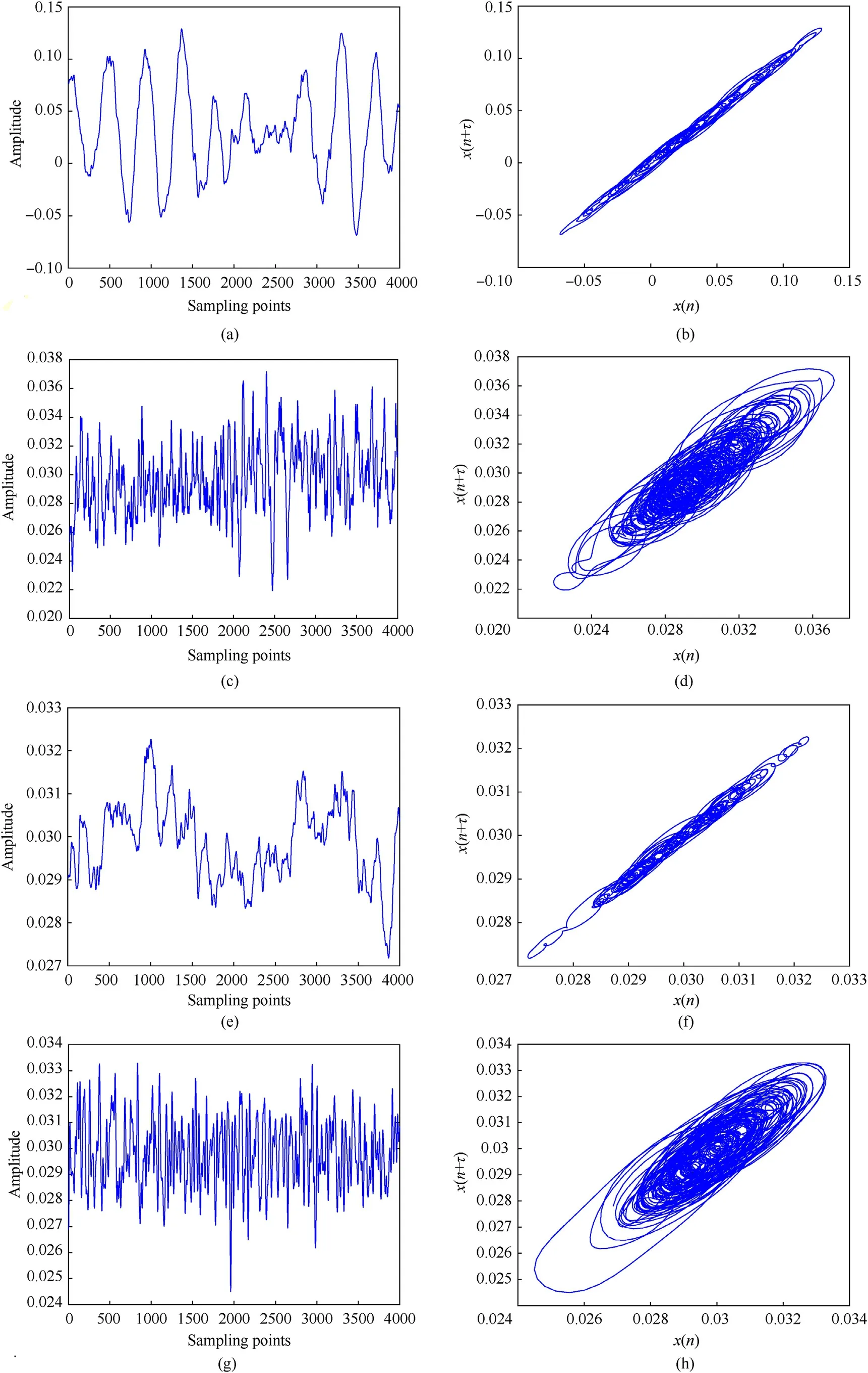
Fig.21.The time domain diagram and phase diagram of four kinds of ship signals after denoising: (a) and (b) S-1; (c) and (d) S-2; (e) and (f) S-3; (g) and (h) S-4.
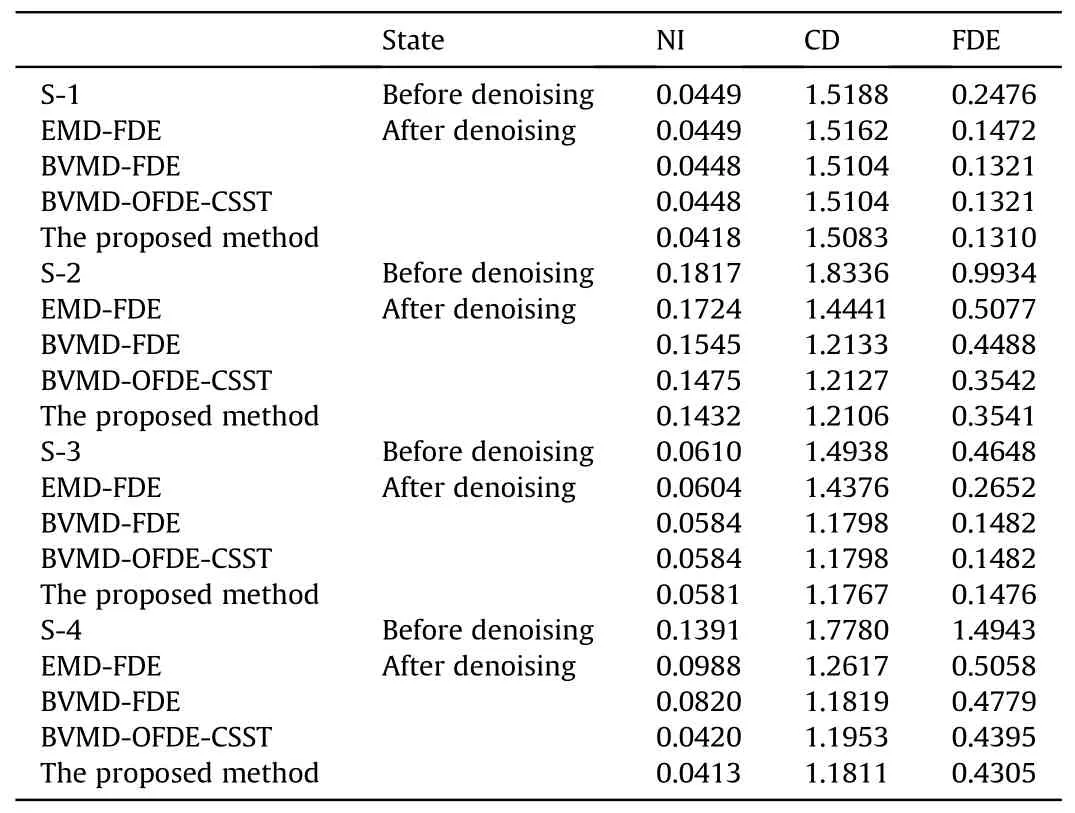
Table 13Evaluation indexes of ship signal before and after denoising.
(1) Lorenz system
where b =10,p =28,f =8/3.Set step size is to 0.01,starting point x0= - 1, y0=0 and z0= 1.
(2) Chen system
where b = 35, p=3 and f = 28.Set the step size to 0.01, starting point x0= - 1, y0=0 and z0= 1.
(3) Rossler system
where b =0.2,p=0.2 and f =9.0.Set the step size to 0.1,starting point x0= - 1, y0=0 and z0= 1.
Select 3000 sampling points of x component of three kinds of chaotic signals as simulated chaotic signals, and add 10 dB noise respectively.Decompose Lorenz signal, Chen signal and Rossler signal with 10 dB noise by BVMD, and calculate the FDE value of each IMF separately.The time domain diagrams of Lorenz signal,Chen signal and Rossler signal are shown in Fig.5(a),Figs.5(c)and 5(e) respectively, and the decomposition results of BVMD are shown in Figs.5(b), 5(d) and 5(f) respectively.Table 4 shows the results of FDE values.
Set the initial threshold of FDE to 0,and the step size to 0.05.The threshold change range is[0,2.6].If the value of FDE is less than the set threshold,reconstruct corresponding components to obtain the recombined signal, and calculate the SNR.Fig.6 shows the change of SNR of different signals with threshold values.
As shown in Fig.6,with the increasing of FDE threshold,the SNR of Chen signal, Lorenz signal and Rossler signal increases continuously, and then decreases after reaching a certain level.When the threshold of Chen signal is(0.70,1.35),the SNR keeps the maximum value.When the threshold of Lorenz signal is (0.55,1.15), the SNR keeps the maximum value.When the threshold of Rossler signal is(0.85,1.50), the SNR keeps the maximum value.Take the intersection of the three signals, that is, when the threshold is (0.85,1.15),the SNR of the three signals will remain at the highest level.Therefore,the threshold of FDE is set as the average of 0.85 and 1.15 in this paper, that is η = 1.
4.3.CS threshold selection experiment
Select three typical chaotic signals, choose 3000 sampling points of x component of three chaotic signals as simulated chaotic signal, and add white Gaussian noise with SNR of 0, 5,10,15 and 20 dB respectively.Decompose noisy chaotic signal by BVMD respectively, calculate the values of CS, and sort CS values from largest to smallest.The CS value of each IMF after three kinds of noisy signals are decomposed by BVMD is shown in Table 5.The CS change curves of noisy Lorenz Signal, Chen Signal and Rossler Signal are shown in Figs.7(a)-7(c) respectively.
As shown in Fig.7, for three different chaotic signals, their CS values will reach a steady state after reaching a certain point, or their slopes will hardly change.Calculate all CSST values according to Eq.(32), and the CSST values of three kinds of noisy signals are shown in Table 6.
From Fig.7,we can easily observe the corresponding IMF order when we reach the stationary point.According to the stationary point,we find the CSST value corresponding to Table 6 and mark it in green.When the value range of CSST is[0.02,0.155],it can meet the stationary demand of noisy Lorenz signal;when the value range of CSST is[0.015,0.027],it can meet the stationary demand of noisy Chen signal; when the value range of CSST is [0.011, 0.022], it can meet the stationary demand of noisy Rossler signal.Take the intersection of the three value ranges,that is,when the value range of CSST is [0.02, 0.022],all the stationary points marked above are satisfied.Therefore,this experiment defines the value of stationary condition φ in CSST as φ = 0.02.
4.4.Chaotic signal denoising experiment
Select three typical chaotic signals, choose 3000 sampling points of x component of three chaotic signals as simulated chaotic signal,and add white Gaussian noise with SNR of 0 dB,5 dB,10 dB,15 dB and 20 dB respectively for chaotic signal denoising experiment.
To show the denoising effect of the proposed method,use EMDFDE, BVMD-FDE and BVMD-OFDE-CSST to compare with the proposed method.Define EMD-FDE, BVMD-FDE and BVMD-OFDECSST as method 1, method 2 and method 3 respectively for easy identification.
Method 1 and method 2 are to decompose noisy signal by EMD and BVMD separately, and calculate the FDE value of each IMF.According to the threshold of FDE (threshold η = 1), distinguish signal IMFs and noise IMFs, and reconstruct signal IMFs to obtain the denoised signal.Method 3 is to decompose the noisy signal by BVMD, and calculate the FDE value and CS value of each IMF.According to OFDE and CSST distinguish pure IMFs, mixed IMFs and noise IMFs,and reconstruct pure IMFs to obtain the denoised signal.The proposed method is to reconstruct pure IMFs and mixed IMFs in method 3, decompose the reconstructed signal by BVMD again,calculate the FDE value of each IMF,and remove noise IMFs by the value of FDE (threshold η = 1) to obtain the denoised signal.
The above noisy chaotic signals are denoised by four methods.Use SNR and RMSE as evaluation criteria before and after denoising.Table 7 shows the denoising results.
Through the experiment of chaotic signal denoising, find that BVMD-FDE has better denoising effect than EMD-FDE, which fully shows that BVMD is more sufficient than EMD.BVMD-OFDE-CSST can distinguish pure IMFs, mixed IMFs and noise IMFs.After denoising, the SNR of the proposed method keeps the maximum and RMSE keeps the minimum, which indicates that secondary decomposition denoising can further remove noise.In order to show the denoising process more intuitively, analyze the 10 dB noisy Lorenz signal in detail.The time domain diagram of noisy and noiseless Lorenz signal are shown in Fig.8(a) and the phase diagram is shown in Fig.8(b).The result of BVMD, the frequency domain diagram and the variation curve of fitness value are shown in Fig.9(a)-9(c)respectively.The result of EMD and the frequency domain diagram are shown in Fig.10(a) and 10(b) respectively.
As shown in Fig.8, the time domain diagram and the phase diagram of the noisy Lorenz signal are extremely complex.As shown in Fig.9,BMVD decomposes the noisy Lorenz signal into 11 IMFs, and there is basically no mode mixing, and the fitness curve remains at a low stable value, indicating that the noisy Lorenz signal has been fully decomposed.Fig.10 shows the decomposition result and frequency domain diagram of EMD.Table 8 shows the FDE value and CS value.Fig.11 shows the change of Otsu value and CS value.
From Table 8,the FDE values of IMF1,IMF2,and IMF3 are all less than 1.Therefore, method 1 selects IMF1, IMF2, and IMF3 as effective components for reconstruction.As shown in Fig.11(a),the variances between entropy classes of IMF1, IMF2, IMF3, IMF4 and other IMFs are the largest, indicating that IMF1, IMF2, IMF3, and IMF4 are closer to useful signal.As shown in Fig.11(b), the CS reaches a stable state in IMF4 by the calculation of Eq.(32).The CS value of IMF4 is 0.1193,which is the threshold of CS,indicating that IMF1, IMF2 and IMF3 are more similar to the original signal.
IMF1,IMF2,and IMF3 are judged to be pure IMFs,and IMF4 is a mixed IMF.Therefore, IMF1, IMF2 and IMF3 are the useful IMFs of method 2.IMF1, IMF2, IMF3 and IMF4 are useful IMFs of the proposed method.Decompose reconstructed signal by BVMD again,then calculate the FDE value of each IMF and remove IMFs with FDE value greater than 1 to get the final denoised signal.Table 9 shows the FDE value of each IMF after secondary decomposition by BVMD.The secondary decomposition result of BVMD, the frequency domain diagram and the variation curve of fitness value are shown in Figs.12(a)-12(c) respectively.Figs.13-15 separately show the time domain diagram and local detail diagram before and after denoising by method 1, method 2, method 3 and the proposed method.
From Figs.13-15,the denoising effect of method 1 is the worst,which is caused by mode mixing during EMD.Methods 2 and 3 remove most of the noise and roughly restore the signal waveform.However, there is still distortion in local details.This is because primary decomposition is not thorough enough, and some IMFs contain a small amount of noise components.The waveform of the proposed method is the closest to that of the noiseless Lorenz signal.It shows that secondary decomposition has a good denoising effect and can further remove noise.The denoised phase diagrams of methods 1, 2, 3 and the proposed method are shown in Figs.16(a)-16(d) respectively.
As shown in Fig.16, the denoising effect of the phase diagram after denoising by four methods can also be clearly seen.The denoising effect of method 1 is the worst, and the trajectory of attractor phase diagram is seriously entangled after denoising.The attractor phase diagram of methods 2 and 3 are improved compared with that of method 1.The geometric structure of the phase diagram is more regular and the curve becomes smooth,but there are still curves entangled in the detail of the attractor phase diagram.The attractor phase diagram of the proposed method is the smoothest, the strongest geometric regularity, and the denoising effect in the detail is better than that of other methods.
4.5.Underwater acoustic signal denoising experiment
In this section,select four different underwater acoustic data to verify the denoising effect.Underwater acoustic data comes from four kinds of ship signals acquired by ocean sonics icListen AF hydrophone (https://github.com/irfankamboh/DeepShip).Besides ship signals,the signals recorded by hydrophones also have natural background noise,noise from marine mammals and noise from any other human activities.Select four different types of ship signals:Cargo,Passenger ship,Tanker and Tug.The above four kinds of ship signals are defined as S-1, S-2, S-3 and S-4 respectively.In this section, select S-4 signal to introduce four denoising methods in detail.Table 10 shows four types of ship signals used in the experiment.Fig.17 shows the time domain diagram and phase diagram of four kinds of ship signals before denoising.Fig.18 shows the decomposed result and frequency domain diagram of S-4 by EMD and BVMD.
From Fig.18, the S-4 signal is decomposed by EMD and BVMD,and 11 IMFs and 10 IMFs are obtained respectively.Calculate the FDE value and CS value of each IMF.Table 11 shows the calculation results.Fig.19 shows the change of Otsu value and CS value.
As shown in Table 11,after S-4 is decomposed by EMD,the FDE values of IMF1,IMF2 and IMF3 are greater than 1,which is the noise IMFs.Reconstruct the remaining components to obtain the denoised signal of method 1.After S-4 is decomposed by BVMD,the FDE values of IMF1 and IMF2 are less than 1.Reconstruct IMF1 and IMF2 to get the denoised signal of method 2.
CSST = 0.0468 is calculated by Eq.(32).From Fig.19(b), IMF1,IMF2, IMF3 and other IMFs have the largest variance between classes.Therefore,it is judged that IMF1 is pure IMF,and IMF2 and IMF3 are mixed IMFs.IMF1 is the denoised signal of method 3.Reconstruct the IMF1, IMF2 and IMF3 to obtain primary denoising signal.Decompose primary denoising signal by BVMD again, and calculate the FDE value of each IMF.The FDE values of IMF3 and IMF4 are both greater than 1 so as to be removed.Reconstruct the residual IMFs to obtain the final denoised signal of the proposed method.The FDE values of each IMF after secondary decomposition are shown in Table 12.Fig.20 shows the results of secondary decomposition and frequency domain diagram by BVMD.The time domain diagram and phase diagram of four kinds of ship signals after denoising are shown in Fig.21.
As shown in Figs.17 and 21,after denoising of four kinds of ship signals,the time domain waveform changes from chaos to clear and regular.The phase diagram changes from twists and turns to more regular and smooth.It shows that the proposed method can effectively remove the ocean noise and restore the real ship signal.NI, CD and FDE value of four kinds of ship signals before and after denoising are shown in Table 13.
As shown in Table 13, four denoising methods can improve the evaluation index of signal,and the proposed method is the best.The above experiments and results show that the proposed method can effectively remove the noise in real underwater acoustic signal.
5.Discussion
(1) BVMD proposed in this paper is to optimize VMD by BWOA.It solves the problem of blindly setting parameters and achieves a good decomposition effect.However, BVMD is inefficient.In the future research,on the premise of ensuring the accuracy of the optimization results, we will devote ourselves to improving the running efficiency of the algorithm.
(2) OFDE proposed in this paper is to FDE threshold improved by Otsu method, which can effectively identify useful signals and avoid the error caused by manually setting the threshold.However,when OFDE is used to set the threshold of high SNR signal, there will be some deviations.In the future, we will study the internal relations of signal to reduce these deviations.
(3) Through above experiment and analysis, it shows that the noise signal may also contain useful information.We directly remove the noise signal, which may cause some useful signals to be lost.In the future, we can extract useful information from noise signal and get better denoising effect.
6.Conclusions
In this paper, a new denoising method of underwater acoustic signal is proposed.The main conclusions are as follows:
(1) Optimized VMD by black widow optimization algorithm,named BVMD, is proposed.It effectively solves the problem of parameter setting of decomposition layer K and penalty factor α.
(2) Fluctuation-based dispersion entropy threshold improved by Otsu method, named OFDE, is proposed.Cosine similarity stationary threshold, named CSST, is proposed.OFDE and CSST can effectively avoid the error caused by manually selecting threshold.
(3) We found that primary decomposition has the problem of insufficient decomposition, and secondary decomposition can make up for the deficiency of primary decomposition and further remove noise.
(4) The proposed method BVMD-OFDE-CSST-BVMD-FDE is compared with EMD-FDE, BVMD-FDE, BVMD-OFDE-CSST.Experimental results show the proposed method can better remove noise.
Declaration of competing interest
The authors declare that they have no known competing financial interests or personal relationships that could have appeared to influence the work reported in this paper.
Acknowledgements
This work was supported by the National Natural Science Foundation of China (Grant No.51709228).
- Defence Technology的其它文章
- The dynamic response and damage models of rebar reinforced polymer slabs subjected to contact and near-field explosions
- Study of the axial density/impedance gradient composite long rod hypervelocity penetration into a four-layer Q345 target
- Active learning accelerated Monte-Carlo simulation based on the modified K-nearest neighbors algorithm and its application to reliability estimations
- Dynamic compressive response of porcine muscle measured using a split Hopkinson bar system with a pair of PVDF force transducers
- Damage of a large-scale reinforced concrete wall caused by an explosively formed projectile (EFP)
- Air target recognition method against ISRJ for radio frequency proximity sensors using chaotic stream encryption

