Influences of across-strike heterogeneous viscosity on the earthquake cycle in a three-dimensional strike-slip fault model

Peng Zhi ,Feng Li ,Jinshui Hung,c,＊

a Mengcheng National Geophysical Observatory,School of Earth and Space Sciences,University of Science and Technology of China,Hefei,230026,China

b Jiangsu Earthquake Agency,Nanjing,210014,China

c CAS Center for Excellence in Comparative Planetology,Hefei,230026,China

Keywords:Across-strike viscosity variation Friction law Power-law rheology Earthquake cycle Asymmetric interseismic deformation

ABSTRACT Geodetic observations have shown that there exist large differences in the viscosity of the deep lithosphere across many large strike-slip faults.Heterogeneity in lithospheric viscosity structure can influence the efficiency of stress transfer and thus may have a significant effect on the earthquake cycle.Until now,how the lateral viscosity variation across strike-slip faults affects the earthquake cycles is still not well understood.Here,we investigate the effects of across-strike viscosity variation on long-term earthquake behaviors with a three-dimensional strike-slip fault model.Our model is a quasi-static model which is controlled by the slip-weakening friction law and powerlaw rheology.By comparing with the reference case,we find that low viscosity on one side of the fault results in a smaller rupture area but with a higher Coulomb stress drop on the ruptured fault region.In addition,low viscosity also leads to a small Coulomb stress accumulation rate.These combined effects increase the earthquake recurrence interval by approximately 10%and the earthquake moments by about 30%when the low viscosity is related to a geothermal gradient of 30 K/km.In addition,across-strike viscosity variation causes asymmetric interseismic ground surface deformation rate.As the viscosity contrast increases,the difference in the interseismic ground surface deformation rate between the two sides of the fault gradually increases,although the asymmetric feature is not pronounced.This asymmetry of interseismic ground deformation rate across a strike-slip fault is supposed to result in asymmetric coseismic deformation if the long-term plate motion velocity is invariant.As a result,this kind of asymmetry of interseismic deformation may influence the evaluation of potential earthquake hazards along large strike-slip faults with lateral viscosity contrast.

1.Introduction

Numerical modeling of earthquake cycles provides a physics-based framework to study the long-term earthquake source processes,thus becoming a fast-growing subject in earthquake science.As a result,a lot of numerical codes based on boundary-element,finite-element,and finite-difference methods have been developed during the recent two decades(e.g.Allison and Dunham,2018,2021;Barbot,2021;Jiang et al.,2022 and references therein;Lapusta and Liu,2009;Liu et al.,2020).To capture all phases of earthquake faulting,from tectonic loading to earthquake nucleation,propagation,and termination,Earthquake cycle models incorporate geological structure,rock properties,friction,or/and rheology of a fault zone,and produce the pre-,inter-,and post-seismic slip and the resulting stress redistribution (e.g.Lapusta and Liu,2009).The framework of earthquake sequence modeling,combined with geological,geophysical and geodetic observations,is adopted in settings like subduction zones,collision zones,and induced seismicity to study fault frictional properties,tremor and slow slip,foreshock and aftershock sequences,and characteristics of small and large earthquake rupture(Allison and Dunham,2018,2021;Barbot et al.,2012;Jiang and Lapusta,2016;Lapusta et al.,2000;Li and Liu,2021;Rice,1993;Tse and Rice,1986).

Physics-based numerical simulations of earthquake cycles can depict fault slip,stress drop,earthquake recurrence and postseismic deformation self-consistently.Conducting these simulations can help us better understand long-term earthquake preparation and thus contribute to earthquake prediction.Using an integrative and fully dynamic earthquake model of the Parkfield segment of the San Andreas Fault,Barbot et al.(2012) produced an earthquake sequence similar to the observed Parkfield earthquake sequence with constraints from geophysical and geodetic observations such as seismicity,GPS movement and InSAR deformation.Although their models could not capture the full range of physical processes,their numerical model did produce a wide range of seismic activity at the Parkfield segment of the San Andreas Fault (Barbot et al.,2012).Similar simulations were also conducted for the Longmen Shan Fault in China (Zhu and Zhang,2013) and the East Japan subduction zone (Weng and Huang,2016).The results from 2D viscoelastic finite element models showed that with proper choices of the viscosity contrast across faults and fault geometry,earthquake cycle models could generate interseismic and coseismic deformation as well as the earthquake recurrence frequency reasonably (Weng and Huang,2016;Zhu and Zhang,2013).Numerical modeling,combined with observational and laboratory techniques,opens a way to develop physical models of earthquake cycles with potential predictive power.

Many geodetic observations show that the coseismic and postseismic deformations are asymmetric across the fault (Fialko,2006;Jolivet et al.,2008;Liu et al.,2019;Malservisi et al.,2001),and one possible mech-anism is suggested as the difference of the substrate viscosity across the fault even though other explanations such as differences in elastic stiff-ness or elastic plate thickness have also been proposed (Liu et al.,2019;Malservisi et al.,2001;Vaghri and Hearn,2012).Detailed studies on the postseismic deformation of large earthquakes strongly support the exis-tence of lateral viscosity contrast across major earthquake faults (Diao et al.,2018;Li et al.,2022;Liu et al.,2019;Pollitz,2015;Pollitz et al.,2017;Weng and Huang,2016).Joint afterslip and postseismic relaxation modeling of the GPS time series up to one decade following the Hector Mine earthquake reveals a significant viscosity variation across the San Andreas fault system (Pollitz,2015).The steady-state viscosity contrast of the lower crust and upper mantle between the northeastern and the southwestern regions could be as high as 4 times (Pollitz,2015).Studies based on the post-deformation of the 2016MW7.0 Kumamoto earth-quake also showed that the transient viscosity of the upper mantle under the forearc zone on the southeastern side is～ 1018Pa s and that on the northwestern side is～ 2.7 × 1018Pa s(Pollitz et al.,2017).Diao et al.(2018) even suggested that the difference in the steady-state viscosity of the lower crust across the Longman Shan fault could reach two magni-tudes based on the seven years post-seismic GPS data after the Wenchuan earthquake.On studying the deformation of the 2001Mw 7.8 Kokoxili earthquake,Liu et al.(2019) concluded that the large asymmetry in the postseismic deformation indicated an across-strike heterogeneous lower crust beneath the northern Qingzang Plateau,and the viscosity of the lower crust beneath the Qaidam basin was 2–4 times larger than that beneath the Songpan-Ganzê terrane.

The difference in the lithospheric viscosity on the two sides of a fault will affect far-field stress transfer efficiency and may further affect earthquake recurrence intervals and postseismic and interseismic deformations;however,most of the previous earthquake cycle simulations only contained depth-dependent viscoelasticity (Allison and Dunham,2018;Lambert and Barbot,2016),and just a small part of these models include the horizontal viscous heterogeneity (Shi et al.,2020;Weng and Huang,2016;Zhu and Zhang,2013).With an analogous earthquake cycle model which imposes prescribed regular earthquake slips on a fault,Vaghri and Hearn (2012) suggested that the influence of the lateral viscosity contrast on ground surface deformation is not significant.However,using a 2D finite element model,with a slip-weakening friction law on the fault,Weng and Huang [2016] found that the viscous heterogeneity had significant influences on the postseismic deformation of the Tohoku earthquake.In this study,we will extend the 2D model of Weng and Huang(2016)to a 3D model,and employ power-law viscosity,which includes the effects of depth-dependent viscosity,as Allison and Dunham(2018)did.

We formulated a 3D quasi-static finite element viscoelastic model with power-law viscosity,which is used to study the interaction between the deep viscous flow on both sides of the strike-slip fault and fault frictional slip during earthquake cycles.It can simulate the stick-slip behavior of the seismogenic fault,and the creep behavior of the other shallow part of the fault.The advantage of this model is that it can simulate interseismic creep and coseismic slip above the brittle-ductile transition zone and the viscoelastic relaxation of the deeper portion of the model simultaneously.The main purpose of this study is to explore the effect of the across-strike viscosity variation on the earthquake recurrence interval and interseismic ground surface deformation.Our results show that the horizontal variation in lithospheric viscosity across the fault can influence the earthquake recurrence interval,and result in an asymmetric interseismic ground surface deformation although asymmetric phenomena are not significant.In the next section,we will describe our model setup,which is followed by numerical results and a brief discussion.

2.Model setup

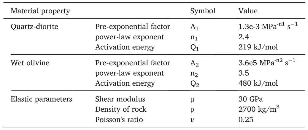
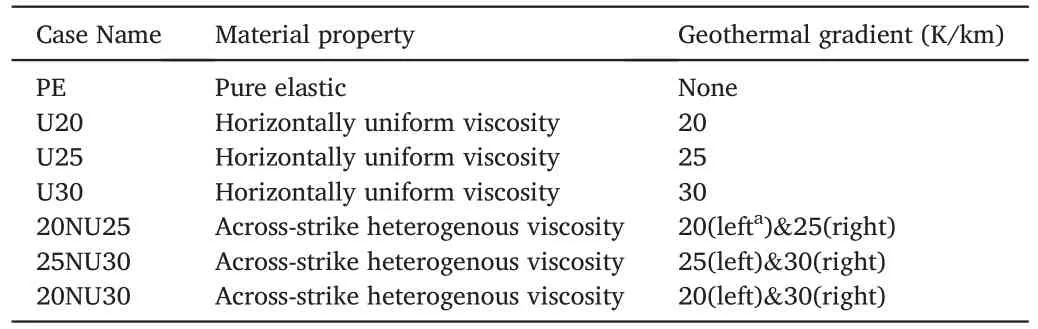
The model here is a three-dimensional model with a left-lateral vertical strike-slip fault embedded in the middle (Fig.1).The fault plane (in gray shadow,Fig.1a) cuts through the entire model domain,and a buried seismogenic zone is located in the upper part of the fault plane (light blue region,Fig.1a).The far-field tectonic loading is imposed by applying a constant relative velocity,Vpl(10-9m/s),on the side boundaries parallel to the fault (blue arrows,half on each side,Fig.1a).Except for the bottom boundary,all other boundary surfaces are free.The bottom boundary is set to be a free slip,which means both the tangential stress and the normal velocity along the boundary surface are zeros.The model is 30 km,15 km and 40 km in length,width and depth,respectively.The range of the seismogenic zone on the 2D fault plane is set as -5 km

2.1. Rheological parameters

The rheology of the material employed here is similar to that used in Allison and Dunham (2018),and the viscoelastic response of lithospheric rocks occurs in the form of dislocation creep.The effective viscosity is stress-and temperature-dependent,and the power law rheology is defined as,

where A is the pre-exponential factor，σ is the differential stress,n is the power-law exponent,Q the activation energy,R the universal gas constant and T is temperature.It is assumed that the crust is composed of quartz diorite,the upper mantle is composed of wet olivine,and a linear transition occurs at the depth from 25 km to 35 km(Fig.1d).The power law parameters in Equa.(1)are controlled by the following equations:

Where φ1and φ2are the volume fraction of the quartz diorite and wet olivine respectively(Fig.1d),and rheology parameter values are listed in Table 1.

Fig.1.(a) 3D model geometry.(b) The initial stress on the fault interface.The static shear stress (τs) in the seismogenic zone,dynamic shear stress (τd),and effective normal stress (σn) are in the solid line,dotted line,and dashed line,respectively.(c) Temperature profile from different geothermal gradients.The solid,dashed,and dotted lines are derived with gradients of 20 K/km,25 K/km,and 30 K/km,respectively.(d)Volume fractions for the quartz-diorite (φ1,solid) and wet olivine (φ2,dotted) used in the mixing law for lithospheric compositions (Ji et al.,2003).(e) The effective viscosity from power law (Allison and Dunham,2018) with the temperature profiles in (c),lithosphere compositions in (d),and a reference strain rate of 10-14/s.

Table 1Rheology parameters (Adapted from Allison and Dunham (2018)).

In our model,the temperature-dependent viscosity is estimated with given geothermal gradients.As suggested in previous numerical experiments (Allison and Dunham,2018),we employ three reasonable values(20 K/km,25 K/km,and 30 K/km)of geothermal gradients,respectively(Fig.1c and Table 2).The effective viscosities calculated based on the above equations with a reference strain rate of 10-14s-1are shown in Fig.1e.In our model,the surface temperature is set to 293 K(20°C).To explore the influence of across-strike viscosity variation on the earthquake cycles,seven cases with different settings are calculated and analyzed in this study(Table 2).

Table 2Cases used in this study.

2.2.Initial fault stress and frictional parameters

Both slip-weakening and rate-and-state friction laws are used in earthquake cycle numerical simulations pervasively (Allison and Dunham,2018;Weng and Huang,2016).In quasi-static simulations,the details of the coseismic slip cannot be captured and variations of the slip rate on the fault usually are not very large and just a few powers of 10.In this case,the velocity-dependent weakening in rate-and-state friction law can be approximated by slip weakening (Uenishi and Rice,2003).Therefore,for computational efficiency,the simple slip-weakening friction law is employed in this study.In the numerical model,the fault behavior(slip and stick)is determined by the balance between the shear stress and the fault strength controlled by the slip-weakening friction law(Ida,1972).The slip-weakening friction criterion is expressed as:

where μsand μdare the static and dynamic friction coefficient,respectively,Dcis the characteristic slip distance and D is the cumulative slip distance during the weakening process,which is reset to 0 after each single rupture.The normal stress and hydrostatic pressure are defined as,

where z is depth,ρ is the density of the material,gis the acceleration of gravity and Ppis the pore fluid pressure.

The dynamic shear stress equals μd＊σn(dotted line,Fig.1b),and the static shear stress equals μs＊σn(solid line,Fig.1b).The static and dynamic friction coefficients are set to be 0.60 and 0.55 within the seismogenic zone,respectively.In the other area of the fault plane,i.e.,the creeping zone,both the static and dynamic friction coefficients are set to be 0.55,which implies that the stress drop is always zero outside the seismogenic zone on the fault plane.In this study,the characteristic slip distance Dcis set to 1 m.It should be noted that it is still a difficult endeavor to determine the value of Dcon natural faults,and the estimated values from a few earthquakes vary from～0.3 m to～5.0 m (e.g.Chen and Yang,2020;Galetzka et al.,2015).In quasi-static earthquake cycle simulations,the most important parameters in the frictional law(equation (5)) are the static and dynamic friction coefficients,while Dcis not important because it is mainly related to dynamic rupture propagation in spontaneous rupture models.However,as we will see later in our model results,the seismogenic zone does not rupture at the same time,but gradually from edge to center,and the Dcvalue affects this process.Thus,a small slip weakening distance is preferred,and it should at least be smaller than the coseismic slips (which is～2 m in our model,refer to section 3.1).In the numerical simulation,a small characteristic slip distance requires a small grid size on the fault to obtain a convergent numerical solution,thereby increasing the computational cost.Our choice is slightly larger than that used in numerical simulations of dynamic rupture models (Chen and Yang,2020;Weng and Yang,2018;Weng et al.,2016;Yao and Yang,2020) to save computational costs for our 3D models.

The mesh size of the fault plane in this study is set to be Δx=500 m,and the dimension of the seismogenic zone is 10 km × 10 km (Fig.1a).Even though we do not want to capture the detailed rupture process of an earthquake in our quasi-static simulation,we still want to see the process before an earthquake event as mentioned in the previous paragraph.This pre-earthquake process requires a high resolution similar to that in dynamic rupture simulation (Weng and Huang,2015,2016);therefore,here we make a simple estimate of our model geometry based on theoretical analysis of Uenishi and Rice (2003) and Day et al.(2005) which are used for dynamic rupture simulations.With parameter values used in this study,the estimation shows that the minimal nucleation size is～7 km and the size of the cohesive zone is about 5 times of our mesh size,which means the setup of our model even fulfills the stricter requirement for coseismic dynamic rupture simulations.These requirements can guarantee the earthquake-like sudden slips happening in our quasi-static simulations of the earthquake cycles,and we can also observe obvious preseismic acceleration phenomenon in the pre-earthquake slip zone,even though we cannot simulate the detailed acceleration process before the coseismic slip.To save computational costs,we use a nonuniform tetrahedral unstructured mesh.The size of the mesh outside of the fault increases with the distance from the fault plane horizontally,and the maximum size of the mesh is 5 km.Our quasi-static simulations of earthquake cycles are performed with the open-source software Pylith(Aagaard et al.,2013).

3.Results

Due to the far-field velocity loading applied in our models,there is some spin-up time required to reach a steady state for analysis of the results.After the spin-up period,all cases with different material properties produced quasi-periodic earthquake cycles.In this section,we present the cumulative slip,viscous strain,viscosity,and Coulomb stress evolution on the fault plane for different cases in order to analyze the basic characteristics of the earthquake cycles.After presenting the results of pure elastic and horizontally uniform cases,which are similar to the prior results from the 2D anti-plane model(Allison and Dunham,2018),we will discuss the simulation results of the cases with across-strike viscosity variations in detail.

3.1.Cumulative slip and earthquake cycles in a purely elastic model

Case PE is a model with a purely elastic material(Table 2),and Fig.2 gives its cumulative slips and coseismic slips on the vertical along the model center,and maximum on-fault slip rates in the seismogenic zone.Cumulative slips in Fig.2a show a typical cumulative slip pattern of the stick-slip behavior in an elastic model (Weng and Huang,2015).The deep part of the model always keeps slipping stably,and the slip rate is equivalent to the boundary velocity,while the stick-slip behavior regularly occurs within the seismogenic zone (10–15 km).Because of the locking state of the seismogenic zone,the slip velocities on the shallow part of the fault(0–5 km)and the area just below the seismogenic zone are slightly smaller than the boundary velocity(Fig.2a).

Fig.2.Characteristics of earthquake cycles of case PE.(a)Cumulative slip after the spin-up time on the vertical along the model center every 5 years.(b)Coseismic slip of 7 earthquakes in our simulation.The red dashed line shows a 2-m coseismic slip.(c) Maximum on-fault slip rate in the seismogenic zone in the whole simulation time.

Coseismic ruptures and the occurrence time of an earthquake event can be determined from the cumulative slips(Fig.2a).In one earthquake cycle,cumulative slips in the locked part of the fault don't change until an earthquake event happens.As a result,the time when the locked area ruptures define the occurrence time of this earthquake event.The earthquake rupture let the cumulative slips in the locked area be the same as other creeping parts after the event,thus leaving a large gap in the cumulative slip patterns (Fig.2a).The larger the gap,the bigger the coseismic slips.The coseismic slips in our three-dimensional model are the accumulative slip differences between the timestep when an earthquake event happens and the timestep just before the earthquake event.Fig.2b shows the coseismic slips of all 7 seismic events on the vertical along the model center in case PE.The coseismic slip of the first event is very different from the others(Fig.2b)due to the spin-up effects which can be observed from the maximum on-fault slip rate (Fig.2c).The earthquake recurrence intervals of case PE are between 65 and 67 years,and the maximum of the coseismic slip of each seismic event is between 2 and 2.2 m after the spin-up phase(Fig.2a and b).

The occurrences of earthquake events can also be recognized from the maximum on-fault slip rate(Fig.2c).However,it should be emphasized that in our quasi-static simulations,the fast coseismic slip cannot be simulated in high precision,and the maximum on-fault slip rate is very small compared with that in the dynamic rupture model or quasidynamic seismic cycle model,especially for cases with low viscosity.Fig.2c shows the spin-up phase clearly,and the model usually reaches a quasi-static state after two earthquake events.The oscillations of the maximum on-fault slip rate before an earthquake event(Fig.2c)are due to the dislocations happening outside the locked area of the seismogenic zone(Fig.2a and b).

It should be noticed that the coseismic rupture can extend upward to the surface and downward to some extent to keep the slips on the fault interface the same as the boundary movements during one complete earthquake cycle.Because the seismogenic zone or locking area is under the ground surface,the shallow part of the fault interface keeps creeping during the interseismic period,so the surface rupture is smaller than the coseismic rupture inside the seismogenic zone(Fig.2a and b).From now on,we only choose the cumulative slips occurring after the spin-up time(Fig.2a) as the representative plot to discuss the characteristics of the earthquake cycles.

Fig.3.Cumulative slip(left column),The component of viscous strain(middle column)and effective viscosity(right column)for different cases(different rows).(a),(d)and(g)are cumulative slips(blue solid line)and cumulative displacements accommodated by bulk viscous flow(red solid line)on the vertical along the model center every 5 years for cases U20,U25 and U30,respectively.(b),(e)and(h)are the snapshots of the component of the accumulated viscous strain through one earthquake cycle on the Y=0 km cross-section of cases U20,U25 and U30,respectively.(c),(f)and(i)are the effective viscosity at the end of the interseismic period on the Y=0 km cross-section for cases U20,U25 and U30,respectively.The horizontal red dashed lines in (a,d and g) indicate the moho depth (30 km) in the composition mixing law.Black lines in (b,c,e,f,h and i) are isolines with numbers indicating logarithm values.Please note,in (a),to make the cumulative displacements accommodated by bulk viscous flow more readable,the red solid lines are drawn every 15 years.

3.2.Cumulative slip and earthquake cycles in a horizontally uniform model

In this section,we will discuss the basic characteristics of the viscoelastic cases with horizontally uniform viscosities,i.e.,cases U20,U25 and U30,which have viscosities based on geothermal gradients of 20 K/km,25 K/km and 30 K/km,respectively(Table 2).Fig.3 shows the cumulative slip,viscous strain and effective viscosity of all three cases.Because of the viscous effects,the results of case U20 show that although the stick-slip behavior in the seismogenic zone is similar to that of a pure elastic model,the elastic slip at the deep part of the fault interface is significantly smaller than the boundary velocity (blue lines in Figs.3a and 2a).The deficit is the cumulative displacement accommodated by bulk viscous flow (red solid lines in Fig.3a),which is obtained by integrating,i.e.,the xy component of the cumulative viscous strain,over horizontal lines at fixed depth [Allison and Dunham,2021],and it increases with time (red lines in Fig.3a).Fig.3b shows the viscous strain componentof the accumulated viscous strain through one earthquake cycle in the plane perpendicular to the fault interface.Theincrease with depth rapidly at about 20 km depth and has another quick increase near the bottom boundary(Fig.3b).Fig.3c gives the effective viscosity of case U20 at the same profile as that of Fig.3b.

With the increase of geothermal gradient,the decrease of the effective viscosity with depth will be larger (Fig.3c,f and 3i).The results of the cases with smaller viscosity(cases U25 and U30)show that although the regular stick-slip behaviors still happen in the seismogenic zone,the viscous effects already influence the rupture behavior of the seismogenic zone (Fig.3d and g).Because of the small effective viscosity,the deep part of the fault interface does not slip anymore(blue lines in Fig.3d and g).A ductile shear zone is formed on both sides of the fault interface as the dominant way to accommodate far-field plate motion (red lines in Fig.3d and g,and Fig.3e and h).This means that the main deformation mechanism of the lower crust and upper mantle has changed from aseismic slip to distributed ductile deformation.

Fig.4.Snapshots of Coulomb stress on the fault at selected times in the interseismic period for cases PE(the left column,a-d),U20(the second column,e-h),U25(the third column,i-l)and U30(the right column,m-p),respectively.The 0-year snapshot represents the Coulomb stress in the last year of the previous earthquake cycle.

The viscous effects also influence the coseismic rupture extends.With the increase in geothermal gradient,the viscosity of the model decreases more rapidly with depth (Fig.3c,f and 3i),and the position of the brittleductile transition also moves up (Fig.3a,d and 3g),which hinders the deep penetration of coseismic slip (blue lines in Fig.3a,d and 3g)(Allison and Dunham,2021).In the pure elastic model (case PE),coseismic slip extends to a depth of about 25 km (Fig.2a).However,in viscoelastic cases,the maximum depth of coseismic slip,which is con-strained by the bulk viscous flow at the lower part (indicated by red solid lines in Fig.3a,d and 3g,and Fig.3b,e and 3h),is only～20 km for case U30.

Stick-slip behavior of the fault is controlled by the Coulomb stress on the fault plane [e.g.Weng and Huang,2015,2016],and the Coulomb stress is defined as:

where τ and σ are the shear and normal stress on the fault,respectively,and μdis the dynamic friction coefficient on the fault.The evolution of Coulomb stress on the fault plane at selected times during the interseismic period for the model with horizontally uniform materials is shown in Fig.4.The frames marked with “0 years show the stress states of the cases just before the rupture of the seismogenic zones (Fig.4a,e,4i and 4m).And the central low-stress region is the area of the final rupture zone at the next time step.After the rupture of the seismogenic zone,the stresses on the locked faults are released and the Coulomb stresses are almost zeros (Fig.4b,f,4j and 4n).With the constant loading from boundary velocity,the stresses build up gradually again within the locked areas (Fig.4).It should be noted that because the normal stress is depth-dependent on the fault,the critical Coulomb stress within the seismogenic zone is also depth-dependent.From the top (5 km) to the bottom (15 km),the theoretical critical Coulomb stress increases from 4.25 MPa to 12.75 MPa;therefore,the upper part of the seismogenic zone is easier to slip than the lower part (Figs.2a,3a and 3d and 3g).

The seismogenic zone (Fig.1a) does not rupture at the same time because of the distributed Coulomb stress (Fig.4).Following Weng and Huang (2015),A pre-earthquake slip zone is defined as the part of the seismogenic zone that can slip slowly ahead of the earthquake event.Slips occur in the pre-earthquake slip zone because the Coulomb stress reaches the critical value.The other part of the seismogenic zone,which slips before the Coulomb stress reaches the critical value,is named the earthquake rupture zone.Therefore,the central low-stress region in Fig.4a,e,4i and 4m is the earthquake rupture zone,and the other area within the seismogenic zone is the pre-earthquake slip zone.In the preearthquake slip period,whilst slip happens in a partial area of the seismogenic zone,the stress in the seismogenic zone does not be released totally because the neighbor area is still locked.The build-up of Coulomb stresses in the seismogenic zone is not simultaneous but is gradually expanding from its edge to its center (Fig.4).The slips do not occur at the same time in the seismogenic zone (Figs.2a,3a and 3d and 3g).The area near the edge of the seismogenic zone will begin to slip first because the Coulomb stress at the edge of the locked area reaches the critical Coulomb stress earlier.However,during this period,the strain energy accumulated in the entire model is not large enough to rupture the entire fault.Besides,because the Coulomb stress in the shallow part of the seismogenic zone is smaller than that in the deeper part,the preearthquake slip zone is mainly formed in the shallow part of the seismogenic zone.

After 50 years of interseismic stress accumulation,the areas of the pre-earthquake slip zone are similar in different cases (Fig.4d,h,4i and 4p).This means that the accumulation rates of Coulomb stress for different cases in the initial stage of the interseismic phase are similar.However,the areas of the pre-earthquake slip zone or the final earthquake rupture zone are different (Fig.4a,e,4i and 4m).For the pure elastic model,when the Coulomb stress on about one-half of the area(i.e.,pre-earthquake slip zone)within the seismogenic zone reaches the critical Coulomb stress,the entire fault begins to rupture,although the Coulomb stress on the other area(i.e.,earthquake rupture zone)still does not reach the critical value of Coulomb stress at the same time(Fig.4a).For case U30,the pre-earthquake slip zone is much larger or the earthquake rupture zone is smaller compared with the other cases(Fig.4a,e,4i and 4m).The reason is that the viscous effects have influenced the build-up speed of strain energy,which is needed to rupture the whole locked fault.The lower the viscosity,the faster the viscous dissipation of the accumulated strain energy,thus resulting in a longer time (i.e.,the interseismic phase)rupturing the whole fault.

The coseismic slips and recurrence intervals can be evaluated from cumulative slip distribution(Fig.3a,d and 3g)as discussed in section 3.1(Fig.2a and b).The coseismic slips and recurrence intervals are almost identical for cases PE and U20(Figs.2a and 3a),and gradually increase from case U25 to case U30(Fig.3d and g).Careful calculations show that the coseismic slips and recurrence intervals for cases PE,U20 and U25 are very close,which are approximately 2 m and 63–69 years,respectively.But for case U30 with the lowest viscosity,there is a small increase in the amount of coseismic slip,accompanied by a longer earthquake recurrence interval which is between 73 and 79 years.In the study of Allison and Dunham [2018],the influence of viscous effects on the earthquake recurrence intervals is about 10 years.However,because the earthquake recurrence intervals of their 2D model are roughly 370 years,they simply ignored these effects[Allison and Dunham,2018].The differences in the earthquake recurrence intervals in our model are also approximately ten years,but compared with the recurrence time of a few decades in our model,this difference is quite large.

3.3.Cumulative slip and asymmetric viscous structure in an across-strike heterogeneous model

Cases 20NU25,25NU30 and 20NU30 are models with across-strike heterogeneous viscosity (Table 2),which means that in these cases,the viscosity on each side of the fault is derived with different geothermal gradients (Table 2,Figs.1e and 5).Fig.5 shows the cumulative slip(Fig.5a,d and 5g),the viscous strain(Fig.5b,e and 5h)and the effective viscosity(Fig.5c,f and 5i)in a representative earthquake cycle for cases with across-strike heterogeneous viscosity.The coseismic slips are similar to the cases with horizontally uniform viscoelasticity (Fig.3a,d and 3g and Fig.5a,d and 5g),but because the slip accumulations are controlled by the part with lower viscosity,the patterns are more similar to that with larger geothermal gradients (Fig.3a,d and 3g and Fig.5a,d and 5g).For example,the coseismic slips in cases 20NU30(viscosity is derived with a geothermal gradient of 20 K/km and 30 K/km,respectively for each side of the fault)and 25NU30(viscosity is derived with a geothermal gradient of 25 K/km and 30 K/km,respectively for each side of the fault) are both constrained to be shallower than 20 km,which is similar to the uniform case U30 in which the geothermal gradient is 30 K/km(Figs.3g,5d and 5g).

The profiles of viscous strain(Fig.5b,e and 5h)and effective viscosity(Fig.5c,f and 5i) show that with different geothermal gradients,the model results show different viscous strain and different effective viscosity on the two sides of the fault.A larger viscous stain accumulated on the side with lower viscosity,while on the other side with higher viscosity,the viscous strain accumulation is smaller(Fig.5b,e and 5h and Fig.5c,f and 5i).In addition,for the lower viscosity side,because the viscosity decreases with depth (Fig.5c,f and 5i),the viscous strain accumulation increases with depth(Fig.5b,e and 5h).However,on the higher viscosity side,both the viscosity and the viscous strain accumulation have a local smallest value at about 25 km(Fig.5b,c,5e 5f,5h and 5i).

The effective viscosity is not only dependent on the geothermal gradient,but also on the stress;therefore,the actual effective viscosity of a model will be adjusted according to its stress field.For example,the viscosity profiles of cases 20NU25 (Fig.5c) and 20NU30 (Fig.5f) show that the viscosity on the left side in case 20NU30 is higher (the color is much darker)even though the background geothermal gradients are the same for both,indicating that the accumulated stresses in the left side of the two cases are different(Fig.5c and f).Similarly,it can be seen from the viscosity profile of cases 20NU25 and 25NU30 that the viscosity on the left side of case 25NU30(Fig.5c)is significantly greater than that on the right side of case 20NU25 (Fig.5i).Therefore,the accumulated stresses in the two cases are different even though they have the same background geothermal gradient of 25 K/km.

The evolution of Coulomb stress for cases with across-strike heterogeneous viscosity is similar to the cases with horizontal uniform viscoelasticity,except that it is controlled by the side with a larger geothermal gradient or lower viscosity.In the pre-earthquake slip stage,the right side with lower viscosity (Fig.5c,f and 5i) accommodates larger viscous strain (Fig.5b,e and 5h) and the far-field plate motion is mostly accommodated by the viscous flow(red lines in Fig.5a,d and 5g)rather than deep fault slip (blue lines in Fig.5a,d and 5g).Analysis of the earthquake recurrence intervals shows that when the viscosity on either side of the model is controlled by a geothermal gradient of 30 K/km,such as cases U30,25NU30 and 20NU30,compared to case PE and other viscoelastic cases with higher viscosity (U20,U25 and 20NU25),the earthquake recurrence interval increases by～10 years.It can be speculated that the low viscosity on either side of the fault results in an increase in the earthquake recurrence interval(Fig.6),which will be discussed in detail in the next section.

3.4.Influences of viscosity on earthquake recurrence interval and seismic moment

Fig.6a summarizes the counts of earthquake events generated by all cases based on their recurrence intervals.The counts labeled as lower viscosity are from cases U30,25NU30 and 20NU30,i.e.,the cases with at least one side have a viscosity with a geothermal gradient of 30 K/km.The counts from all the other cases are classified as with higher viscosity.The earthquake recurrence intervals with higher viscosity are between 63 and 69 years (blue bars)and those with lower viscosity are between 73 and 79 years (red bars).Obviously,the recurrence intervals are controlled by the lower viscosity side of the model,which means that if the viscosity on either side of the fault is low (determined by a geothermal gradient of 30 K/km),the recurrence intervals will increase to greater than 70 years.Therefore,if the viscosity of either side of the fault decreases,the recurrence interval might be prolonged.

Fig.6.(a) Earthquake recurrence interval for all cases.The red and blue bars represent the statistical results for cases with a different effective viscosity.(b)Seismic moments of earthquakes are generated in all cases.Different symbols represent seismic moments of different cases in different cycles.Blue and red marks represent earthquake recurrence periods less and greater than 70 years,respectively.The green and black dotted lines represent the seismic moments released by earthquakes with magnitudes of MW 6.9 and MW 7.0,respectively.

The seismic moments can be evaluated with the model parameters and coseismic slip,that is,M0=μ A S,where μ is the shear modulus,A is the fault rupture area and S is the average slip of the fault rupture.Fig.6b lists the seismic moments of all earthquake events of all cases used in this paper.It can be seen from Fig.6b that the earthquake moments change with time,especially at the earlier stage,and will approach a stable value at the later stage.These earthquake events can be grouped into two categories:one group with higher viscosity and a moment of～3.2×1019Nm;and the other with lower viscosity and a moment of～4×1019Nm(Fig.6b).The model with lower effective viscosity on either side of the fault,i.e.,cases U30,25NU30,and 20NU30,released higher seismic moments in earthquake events,resulting in earthquakes with a moment magnitude of～7.0(Fig.5b).By contrast,the other cases released lower seismic moments which are equivalent to aboutMW6.9 earthquakes.In order words,the decrease in viscosity will prolong the earthquake recurrence interval and increase the energy released by each earthquake event.

Fig.7.(a)Time evolution of Coulomb stress at a point in fault interface(Y=0 km,Z=-13 km)during one interseismic period for different cases.Black,red,green and blue solid lines are for cases PE,U20,U25 and U30,respectively.Red,green and blue dashed lines represent cases 20NU25,25NU30 and 20NU30,respectively.(b) Zoom-in of (a).

4.Discussion

4.1.Effects of viscosity on earthquake recurrence interval

In order to understand how viscosity variation influences the earthquake recurrence interval,we analyzed the time evolution of the interseismic Coulomb stress.Fig.7 shows the change of the Coulomb stress with time at a point with Y=0 km and Z=-13 km.For all seven cases,the Coulomb stresses at the initial stage of the interseismic phase are almost identical,which is consistent with that shown in Fig.4.However,at the end of each interseismic phase,the Coulomb stresses of different cases are divergent slightly(Fig.7).As the viscosity decreases,the stress accumulation rate decreases a little.As a result,for cases with lower viscosity on either side of the fault,such as cases U30,25NU30 and 20NU30,the earthquake recurrence interval will increase,accompanied by larger coseismic stress drops.

4.2.Asymmetric across-fault interseismic deformation rate

As mentioned earlier,many geodetic observations have shown asymmetric interseismic ground surface deformation for a number of major strike-slip faults and proposed that one possible mechanism for this phenomenon is the lateral viscosity contrast across faults.Our results show that the surface deformation is symmetric for all horizontally uniform cases;but is not symmetric anymore in cases with across-strike heterogeneous viscosity,even though this asymmetry is not very significant.Fig.8 shows the ground surface velocity at different selected times in a representative earthquake cycle for the three cases with across-strike heterogeneous viscosity,i.e.,case 20NU25,25NU30 and 20NU30(Table 2).

Interseismic ground surface velocities on the two sides of the fault for cases 20NU25,25NU30 and 20NU30 along the profile Y=0 km are presented in Fig.8.It can be seen that the velocity on the side with lower viscosity (solid line) is faster.The larger the viscosity contrast is,the larger the velocity difference between the two sides of the model will be.The largest difference is about 2.5%,which is about 1 mm/a(Fig.8e and f)with the parameters used in our model.In practice,this small value is not large enough to explain the observed asymmetric interseismic deformation (Vaghri and Hearn,2012);therefore,other mechanisms to produce asymmetric interseismic deformation around strike-slip faults,such as local elasticity variation(a damage zone)or geometric effects of fault zones(shear zone offset at depth or a dipping fault),deserve further exploration(e.g.Fialko,2006;Jolivet et al.,2008).

It deserves to point out that this paper only discusses the influences of across-strike viscosity variation in a quasi-static numerical model.However,there exist many factors that could affect the earthquake cycle as well as the corresponding coseismic slip(e.g.Weng and Huang,2015;Weng et al.,2016).One factor of particular interest is the shallow low-velocity fault zone which sometimes is termed a damaged fault zone(Yang et al.,2021).Dynamic rupture simulations (e.g.Harris and Day,1997;Huang and Ampuero,2011;Huang et al.,2014;Pelties et al.,2015;Weng et al.,2016) show that the damaged fault zone can modulate earthquake rupture extents,rupture speed and rise time.Results from two-dimensional fully-dynamic earthquake cycle models show that the fault damage zone can amplify coseismic slip and rupture extents to a large extent(Thakur and Huang,2021;Thakur et al.,2020).Quasi-static models of Weng and Huang (2015) show that stress disturbance also influences the size and frequency of earthquake events.Therefore,the study of the influences of viscosity,low-velocity fault damage zone,stress disturbance and their combinations,as well as developing a three-dimensional fully-dynamic earthquake cycle model still needs to be worked on continuously.

Fig.8.Horizontal surface velocity along the profile Y=0 km at selected times during the interseismic period for cases 20NU25 (a) and (b),25NU30 (c) and(d) and 20NU30 (e) and (f),respectively.Solid lines represent values on the right side of the fault (lowviscosity side) and the dashed lines on the left side of the fault (high-viscosity side).The green,blue and red lines are values at the time of 1 year,1/4T and 3/4 T during one interseismic period.(b),(d) and (f) are zoom-ins of (a),(c) and (e),respectively.T is the earthquake recurrence interval.Model velocity values are normalized by half of the prescribed boundary velocity (vpl).

5.Conclusions

We developed a three-dimensional viscoelastic earthquake cycle model,which employs a slip weakening friction law and a power law rheology,to simulate the stick-slip behavior of a strike-slip fault.The results of the cases with horizontally uniform materials are almost the same as that of the previous 2D model (Allison and Dunham,2018);however,our 3D quasistatic finite element model can be used to study the influences of horizontally heterogeneous materials,in addition to self-consistently generating quasi-periodic earthquakes.

The results of the case with pure homogeneous elastic material show that the deep part of the fault always creeps at the same rate as the imposed plate velocity.Forviscoelasticcaseswitha powerlaw rheology,the position of the brittle-ductile transition,which hinders the deep penetration of coseismic slip,gets shallower when the geothermal gradient increases.Compared with the cases with a purely elastic material(case PE)and low geothermal gradients(cases U20 and U25),the case with a high geothermal gradient (case U30) produces earthquake events with longer recurrence intervals(～10%longer)and larger seismic moments(～30%larger).

Results of the cases with across-strike heterogeneous viscoelastic materials showed that the characteristics of an earthquake cycle are mainly controlled by the side with lower viscosity.When the viscosity on either side of the fault is controlled by a geothermal gradient of 30 K/km(cases U30,25NU30 and 20NU30),the earthquake recurrence interval and seismic moments will increase by approximately 10% and 30%respectively,compared to cases with lower geothermal gradient (cases PE,U20,U25 and 20NU25).The viscosity of the off-fault material can affect the stress accumulation rate on fault at the end stage of the interseismic phase,and the main influences are that low viscosity tends to postpone the earthquake occurrence and dissipate some accumulated strain energy.

It is worth mentioning that within the framework of earthquake cycle dynamics,we find that the across-strike lithospheric viscosity contrast does cause asymmetrical ground surface deformation during the interseismic phase.As the across-fault viscosity contrast increases,the difference in the ground surface deformation rate also gradually increases.However,this asymmetry of the ground surface deformation rate caused by the across-strike viscosity contrast only is not significant.As a result,to explain the observed asymmetrical interseismic deformation across many large strike-slip faults,other contributions should be taken into consideration.

Data and resources

All data used in this manuscript are produced with Pylith,which is open-source software and available at: https://pylith.readthedocs.io/en/latest/user/index.html.The finite element mesh of our numerical model is generated with the open-source software Cubit which is available at: https://cubit.sandia.gov/.Figures are plotted with Matlab which is a commercial software.

Author agreement and Acknowledgments

We are submitting the above original research for consideration for publication in your journal.All authors have reviewed the final version of the manuscript and approved it for publication.The authors declare that the work described was original research that has not been published previously and is not under consideration for publication elsewhere,in whole or in part.This work is supported by the National Natural Science Foundation of China(42 074105;92155204)and the Joint Open Fund of Mengcheng National Geophysical Observatory (No.MENGO-202004).We thank Deputy Editor in Chief Z.Peng and two anonymous reviewers for their constructive comments and suggestions that improved this paper.

Declaration of competing interest

We are submitting the above original research for consideration for publication in your journal.All authors have reviewed the final version of the manuscript and approved it for publication.The Authors declare that there is no conflict of interest.