Temperature-free mass tracking of a levitated nanoparticle

Yuan Tian(田原), Yu Zheng(郑瑜),†, Lyu-Hang Liu(刘吕航),Guang-Can Guo(郭光灿), and Fang-Wen Sun(孙方稳)

1CAS Key Laboratory of Quantum Information,University of Science and Technology of China,Hefei 230026,China

2CAS Center for Excellence in Quantum Information and Quantum Physics,University of Science and Technology of China,Hefei 230026,China

Keywords: optical levitation,nanoparticle,mass measurement,thermal desorption

1.Introduction

Nanoparticles are one of the most critical research systems in nanomaterials research.[1–3]Relying on their large surface-to-volume ratio and specialized surface morphology,[4,5]nanoparticles have a wide range of applications in areas including molecular adsorption,[6,7]surface functionalization,[8,9]and catalytic reaction.[10,11]The characterization of particle properties is an essential part of nanoparticle and microparticle research, including the weighing of their mass.[12–22]The mass of a nanoparticle is related to its density, size, fill rate, composition, and other properties that provide important criteria for the identification of nanoparticles.Conventionally,a nanoparticle’s mass is estimated using data on density, particle size analysis, and particle properties measured on a bunch of particle powder.[23–26]This approach gives less accurate information on the mass of nanoparticles.It also lacks information on the individual nanoparticles and does not allow for the analysis of differences in properties,such as density, between nanoparticles in the same batch of samples.

Recently, a number of methods have been invented to measure the mass of individual nanoparticles.[15–17,27–29]Among these mass measurement methods, the scheme using optical levitation is the most promising.Using the calibrated or estimated electric or optical field as a reference, the optical levitation system achieves high-precision fg-level mass measurement of nanoparticles.[16,28,29]A significant reduction in the mass of silica nanoparticles is observed.[12,22,28,30]However,comprehensive investigations of this mass-changing process are still lacking.Considering that the mass of most materials changes with increasing temperature, simultaneous high-precision measurement of the mass and temperature of nanoparticles is essential for investigating their property transitions.Nevertheless, there is still no satisfactory solution for the simultaneous measurement of the mass and center-ofmass motion(COM)temperature.This is because the existing schemes depend on the statistical properties after interaction with a thermal bath of known temperature.Only one of the mass or temperature can be measured, while the other has to be known beforehand.[31,32]Although there are attempts to estimate the particle temperature by using the scattered light intensity and the gas pressure,[12]the accuracy and reliability of the temperature obtained by this method are very poor.

Here we present a scheme for the temperature-free mass measurement of optically levitated nanoparticles with the assistance of a sinusoidal electrostatic driving force.By using a known AC driving force as a reference scale, the involvement of temperature as a known variable in the mass measurement process is no longer needed,thus enabling a temperatureindependent mass measurement scheme.With this scheme,we tracked in real time the variations in mass, COM temperature, and other properties of a 165 nm nominal diameter silica particle as the air pressure changed.Using this scheme,it is possible to investigate the dynamics of nanoparticle properties with temperature,[33,34]for example,the crystalline form transition temperature or melting temperature of the nanoparticles,[35–39]the temperature dependence of the reaction rate with gas molecules,[40]temperature-controlled drug release,[41]etc.

2.Mass measurement method

Consider an optically levitated oscillator driven by a sinusoidal forceFAC.Its mechanical energy variation can be divided into three parts:

with

where dEACrepresents the work done by the AC driving force.xis the position of the oscillator.dEdamprepresents the work done by air damping.Γ0is the air damping coefficient.mis the mass of the nanoparticle.vis the velocity of the oscillator.dEstorepresents the work done by the stochastic force.kBis the Boltzmann constant.T0is the effective temperature which is equal to the COM temperature when the external driving force’s heating(cooling)effect can be neglected.Wrepresents the Wiener process.

Here, dEcan be calculated using the calibrated oscillator trajectory andE=m(v2+Ω20x2)/2,whereΩ0is the eigenfrequency of the oscillator.The schematic diagram of mechanical energy variation dEand the work done by the AC driving force dEACvarying with timetis shown in Fig 1(c).Multiply both sides of Eq.(1)by dEACand integrate,which is

Because the dWis independent of dEAC,dEACdEsto=0.Extracting massmfrom Eq.(3),we have

For a realistic measured oscillator trajectory, the mass of the nanoparticle can be obtained by using the discrete form,which is

where ∆xis the difference of trajectories: ∆x(t)=x(t+∆t)−x(t),∆tis the sampling interval.Γ0is obtained by fitting an exponential equation to the variance of trajectory ensembles.[24]Ω0is obtained during the calibration of the particle’s trajectory, which is shown below.According to the experiment and simulation result,(dEACdEdamp) is much smaller than(dEACdEAC).When the pressure is below 1 mbar,(dEACdEdamp) can be neglected when measuring the particle’s mass.

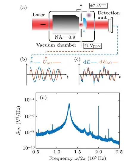
Fig.1.(a)Schematic diagram of vacuum optical levitation.A 1064 nm laser beam is focused by an objective lens (NA = 0.9) to trap the nanoparticle.The forward scattered light is collected by an aspherical lens(NA=0.6)to detect the position of the particles.The driven electric field is generated by a pair of stainless steel rods that are connected to a signal generator.An additional high voltage electrode is used for charge control of the particle.(b) The schematic diagram of particle’s trajectory x (blue line) and driving voltage UAC (orange line) varying with time t.The units of x and UAC shown in the figure are not the same.(c) The schematic diagram of mechanical energy variation dE(blue line) and the work done by the AC driving force dEAC (orange line)varying with time t.(d)PSD of the trajectory of a particle under AC driving force at 1 mbar.The curve was obtained by averaging the PSD of eight trajectories of 1 s duration.The frequency of the driving force is 200 kHz.

3.Experimental method

3.1.Experiment setup

The experimental schematic is shown in Fig.1(a).The nanoparticle to be weighed is optically trapped in a vacuum chamber,where the air pressure can be controlled from atmospheric pressure to high vacuum.The optical potential used to trap the nanoparticle is formed by a tightly focused linear polarization laser,whose wavelength is 1064 nm and the numerical aperture of the objective is 0.9.The forward scattering light is collected by an aspheric lens for the measurement of the particle’s translational movement.Stainless steel rods,which are mounted on both sides of the trapping potential, are used as electrodes for the implementation of the electric field.The distance between the two electrodes is approximately 2 mm.

3.2.Calibration coefficient and oscillation frequency

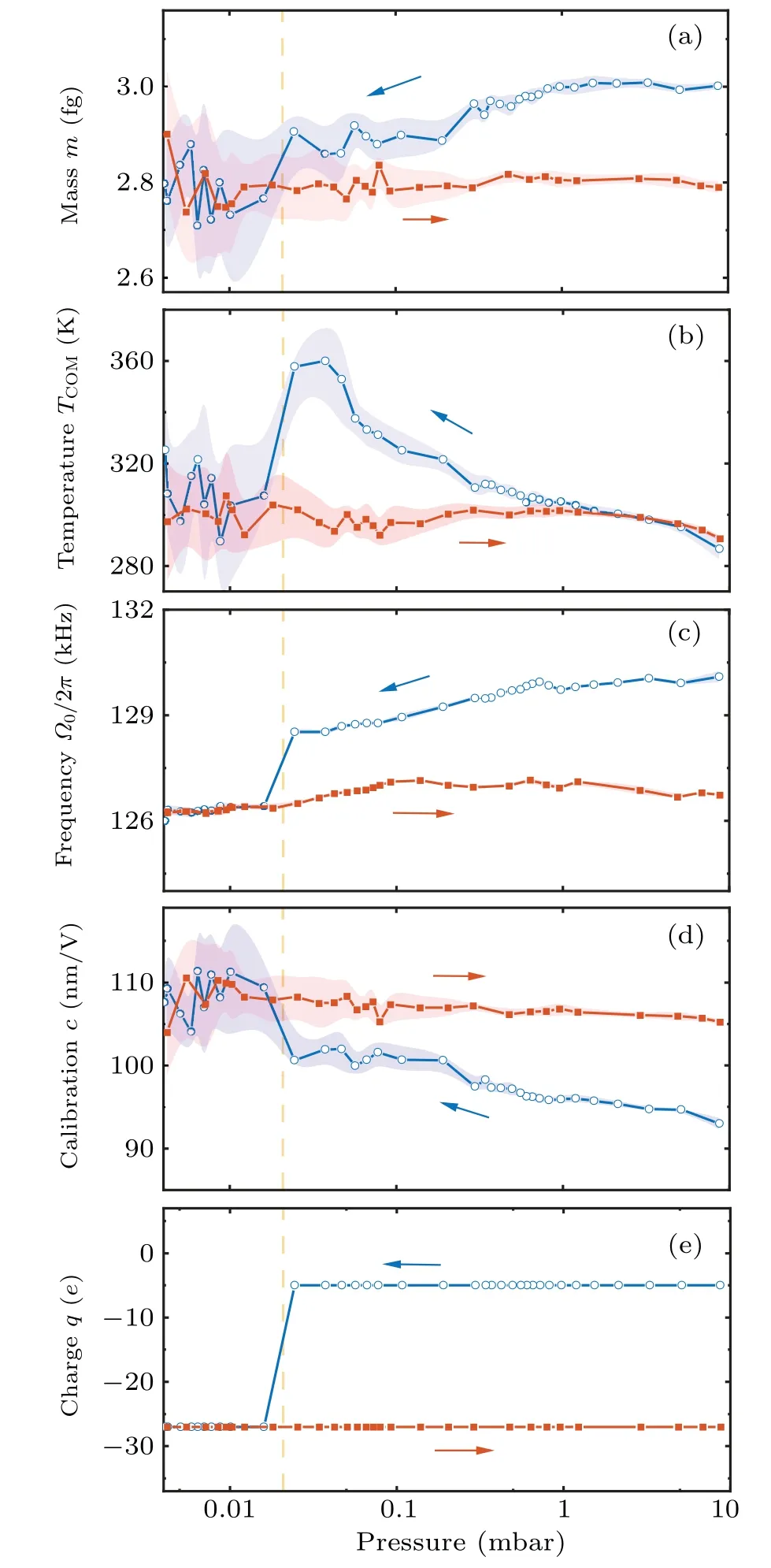
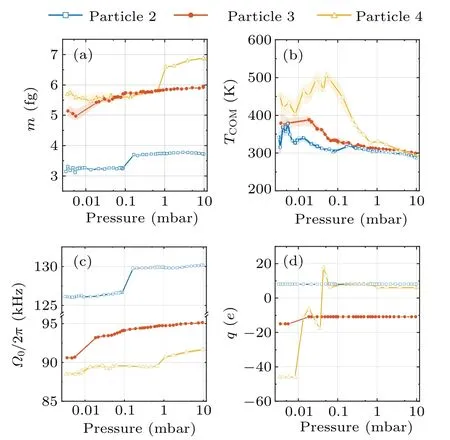
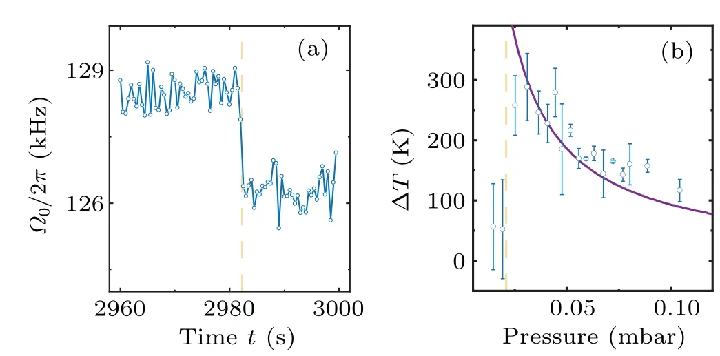
According to Eq.(5),the mass measurement requires the particle’s position calibration coefficientcto convert detected signalVto the particle’s positionx=cV.The calibration of the particle’s trajectory is achieved by the Duffing nonlinearity induced frequency shift analysis of trajectory fragments with different amplitudes.[28,42]First, we collect the detector’s electric signals that satisfyV0−dV

whereΩx0is the eigen frequency atx-axis,andξxis nonlinear coefficient.Therefore, the frequencyΩx0and the calibration coefficientccan be obtained by fitting Eq.(6)to the averaged detection signal.Such a calibration method has high precision at air pressures below 10 mbar.When the pressure is below 10−3mbar, it is hard to levitate the nanoparticle stably without COM temperature cooling.The COM temperature cooling harms the precision of the calibration coefficient.[42]Thus,the applicable pressure range of this calibration method is 10−3mbar–10 mbar,limiting the pressure range of our mass measurement.

3.3.Driving force and charge

In the experiment, two principles are followed in the selection of parameters for the driving force.The first rule is the high signal-to-noise ratio(SNR)of the driven motion component, which can be inferred from a much higher drive PSD peak at the AC driving force frequency than the PSD from thermal motion.Second, the component of motion imposed by the driving force is negligible compared to the total thermal motion.Otherwise,the accuracy of the calibration method based on the Duffing nonlinear analysis of the motion trajectory will be significantly reduced.As shown in Fig.1(d), the frequency of the AC driving force is 75 kHz away from the oscillator’s eigenfrequency.The SNR of the driven motion is about 4.4×105in a trajectory of 1 s duration, and the power of the driven motion compared with the total thermal motion is〈〉/〈x2〉=7.1×10−4.The mass measurement also requires the knowledge of the driving force’s amplitudeFAC.There are two ways to determine the sinusoidal electrostatic driving force.The particle’s mass can be measured with the calibrated thermal equilibrium trajectory and the equipartition theorem.[23]The size of the AC driving force is obtained by the linear response function of the levitated harmonic oscillator[16](not adopted below 10 mbar due to nonlinearities)

whereIis the integral of the PSD of the linear oscillator in an electric field at the driving frequencyΩdr.m10mbaris the particle’s mass measured at 10 mbar.At pressure above 10 mbar,the thermal conductivity is strong enough to keep the nanoparticle at the same temperature as room temperature.[28,31]The particle’s mass can be measured with the calibrated thermal equilibrium trajectory and the equipartition theorem.[23]m10mbar=kBTem/(c2〈V2〉),where〈V2〉is the mean square values of the detected signal,andTemis the room temperature.Γandare obtained from fitting Lorentz line to PSD.In advance,the electric field strength at the particle trapping position is obtained by the electric field force measurements of a particle with a known charge.The AC driving force would be the electric field strength multiplied by the charge.

If the charge change occurs only once during the pressure drop and rise,then the changedFACcan be recalibrated when the pressure returns to 10 mbar.And if the charge change occurs multiple times during mass monitoring, we first assume that the mass of the particle remains constant after one charge change occurs and estimate the charge of the particle by the height of theFACpeak on the PSD.Since the charge can only be an integer multiple of the elementary charge and the mass can only decrease, the change in theFACdue to the charge change can be recovered.However,in the case of large charge changes, theFACestimation for multiple charge changes becomes unreliable.

3.4.COM temperature

After we finish the trajectories’ calibration and driving force estimation, we can get the particle’s mass based on Eq.(5).As we already have the particle’s mass, the particle’s COM temperature can be obtained with the equipartition theorem thatTCOM=mΩ〈x2〉/kB.

4.Experimental results

A nanoparticle,which is a silica nanosphere with a nominal diameter of 165±20 nm(model number: SS02000,Bangs Labs Inc.), is sent into the optical trapping potential by a nebulizer.The nanoparticles are stored in water and diluted with ethanol before delivery.After the nanoparticle has been trapped, the air pressure in the vacuum chamber is reduced to 10 mbar from the atmosphere.After measurement ofFAC,the mass tracking of the nanoparticle starts.Then, the reduction in air pressure in the vacuum chamber restarts at a very low speed.When the pressure reaches below 5×10−3mbar,the pumping stops,and a slow leak into the vacuum chamber begin to bring the air pressure back to 10 mbar.This pressure control process lasts approximately 14400 s.At the same time,the trajectory of the levitated nanoparticle along the electrode direction and the driving electric field signal are recorded.

We notice that the charge change event happens once when the pressure is reduced to 2×10−2mbar.The particle’s charge changes from−5eto−27eas shown in Fig.2(e),which corresponds to an electric field of 6.38 kV/m.

Fig.2.Property changes of the optically levitated nanoparticle during the first pressure pump down and venting cycle.(a)Mass m.(b)COM temperature TCOM.(c)Oscillation frequency Ω0/2π.(d)Calibration coefficient c.(e)Electric charge q.The pressure is reduced from 10 mbar to 4×10−3 mbar for the first time after the particle is trapped and then back to 10 mbar.The blue dots represent the pressure drop process and the orange squares represent the pressure rise process.Each data point is obtained from the average of five 20 s segments of the trajectory.The shading represents the standard deviation of the data.

With the calibrated trajectory and Eq.(4), the nanoparticle’s mass variation with air pressure is obtained,as shown in Fig.2(a).As the pressure is reduced below 1 mbar, the mass of the particle gradually decreases.However,at 0.02 mbar,the mass of the nanoparticle suddenly decreases when the charge change event happens.After that,there is no further significant change in the mass of the particle.The statistical error of the mass measurement,shown in Fig.2(a),mainly comes from the uncertainty of calibration.As the pressure drops, the nonlinear calibration requires a longer trajectory signal to maintain the precision of the calibration coefficients.[42]However,since data sampling of equal-length trajectories is used in the actual experiment, the statistical error of the calibration coefficients increases with decreasing air pressure.

The COM temperature is influenced by both the internal temperature of the particle and the ambient temperature,usually between them.[31]It can be seen from Fig.2(b) that, at the beginning of the vacuum evacuation, the COM temperature rises as the air pressure decreases.This can be explained by the fact that thermal conductivity decreases with decreasing air pressure.However, at 0.02 mbar, where the mass and charge have dramatically changed,the particle’s COM temperature suddenly drops to near room temperature.

Similar to charge, mass, and COM temperature, the calibration coefficient and the oscillation frequency of the nanoparticle change significantly as the air pressure decreases to the transition point(seen in Figs.2(c)and 2(d)).Such a transition pressure point only happens during the first decrease in the air pressure.No similar transition points are observed during subsequent pressure increases or repeated vacuum evacuations.

Fig.3.Property changes of the other three nanoparticles at the first pressure drop.(a)Mass.(b)COM temperature.(c)Oscillation frequency.(d)Charge.The blue squares,orange dots,and yellow triangles represent particles 2,3,and 4,respectively.

Figure 3 shows the results of tracking the changes in the properties of the other three particles during the first pressure decrease.The power of the trapping laser is approximately 350 mW for the particle in Fig.2 and particle 2,and is approximately 180 mW for particles 3 and 4.Although the transition pressure and the magnitude of change are different for different particles,most particles undergo a significant reduction in mass when the air pressure drops below a certain point.Such abrupt changes in mass are usually accompanied by significant changes in COM temperature,calibration coefficients,oscillation frequencies,and electrical charges.

5.Discussion

Since long trajectories are not required,the measurement of the particle frequency provides us with evidence of higher temporal resolution for the abrupt changes in particle properties.As shown in Fig.4(a),the duration of the abrupt change in the mass of the particles in Fig.2 does not exceed 1 s,which corresponds to a relative pressure change of about 0.5%.Since the heating of particles by the laser is inversely proportional to the air pressure in a vacuum environment,[12,28]by fitting the pressure–temperature data of the particle before the abrupt change point(shown in Fig.4(b)),we can obtain that the internal temperature increase of the particle does not exceed 2.5 K at the moment of the abrupt change.The internal temperature of the particle is obtained based on the method in Ref.[32].

Fig.4.(a)Frequency tracking of the particle shown in Fig.2 near the abrupt change point.(b)Temperature difference ∆T between the internal temperature of the particle shown in Fig.2 and the ambient temperature with decreasing pressure.The solid line is the fitting to the data before the abrupt change point.

We can use the experimental results of nanoparticle mass tracking described above to provide a conjecture as to the reason for the changes in the properties of nanoparticles during the pressure decrease.As the silica nanospheres we used are synthesized with the St¨ober process,[43]there would be plenty of water molecules adsorbed on the particle’s surface.Moreover, as the chemically synthesized silica particles are typically amorphous and porous,[44]water molecules can be sealed inside the nanoparticles.As the pure silica’s absorption of 1064 nm laser light is negligible, the heating effect from the trapping laser on the nanoparticles comes mainly from the water molecules they contain.When the thermal conductivity of the system decreases with decreasing air pressure,the nanoparticle’s internal temperature is rising and the water molecules adsorbed on the particle surface is detaching from the particle,which results in a gentle decrease in the particle’s mass.However, as the water that is sealed inside the particle cannot be released,the particle’s temperature continues to rise with decreasing pressure.When the internal temperature of the particle exceeds the boiling point of water, the water inside the particle is boiled into vapor.As the temperature continues to rise, the vapor pressure inside the particle exceeds the upper limit that the particle’s sealing structure can tolerate.Water molecules are expelled from the particle’s crack in the form of steam.The blasted vapor rubs against the particle and brings more charge away with them.The loss of water could introduce a decrease in the oscillator’s eigenfrequency and calibration coefficient which has been confirmed by the experiment.[12,22,28,30]

The sudden loss of the water molecules inside(or on the surface)of the silica nanoparticles cannot be explained by the loss of surface water layers.Because the water molecules are connected through hydrogen bonds which have a large range of bond energies and correspond to a wide range of desorption temperatures.Therefore,the commonly used Zhuravlev model,[45]which is based on hydrogen bond breaking to explain the dehydration process of silica particles, is unable to explain the abrupt mass loss phenomenon found in this work.Such a sudden change cannot be observed by conventional desorption analysis tools, such as thermal desorption spectrometry,[46]because they cannot work with an individual particle,and the properties of desorption vary considerably between different particles.

6.Conclusion

We demonstrate an electrostatic driving force assisted mass measurement method for an individual nanoparticle that does not require the knowledge of temperature.The method can be utilized in the investigation of temperature-dependent mass variation.For example, the observation of molecules desorption from a particle’s surface when the surface temperature is increased.With this method,we monitor the variation of the properties of optically levitated nanoparticles with air pressure,including mass,temperature,electric charge,calibration coefficient,and oscillation frequency.We find that there is a sudden loss of the nanoparticle’s mass when the pressure is decreased below a certain point.This phenomenon cannot be explained by the desorption of water molecules from the surface.This work provides a new tool for surface and structure analysis in nanomaterials science.

Appendix A:Internal temperature measurement

The internal temperature of the particle in Fig 4(b)is obtained based on the method in Ref.[32].When the particle is heated, the heat can be transferred to the colliding gas particle.This causes the difference between the temperature of impinging gas particleTimpand the temperature of the emerging gas particleTem.The relation betweenTimp,Temand the COM temperatureTCOMis

TheTCOMis measured based on the energy equipartition theorem and the measurement result of the particle’s mass.The temperature of impinging gas particles equals the room temperature (293 K in our experiment).Thus, we can obtain the temperature of the emerging gas particle based on Eq.(A1).

The relationship between the gas temperatures and the surface temperature of the particleTsuris given by the accommodation coefficient

The accommodation coefficient is known and close to 0.777.[32]Thus, we can obtain the surface temperature of the particleTsurbased on Eq.(A2).Since the particle is in nano size,the internal temperature of the particleTintwould be the same as the surface temperature.Thus, we can obtain the internal temperature of particleTint.

Acknowledgements

Project supported by the National Natural Science Foundation of China (Grant Nos.12104438 and 62225506),CAS Project for Young Scientists in Basic Research (Grant No.YSBR-049),and the Fundamental Research Funds for the Central Universities.