Effect of low operating temperature on the aerodynamic characteristics of a high-speed train

Xiujuan MIAO, Guangjun GAO, Jiabin WANG, Yan ZHANG, Wenfei SHANG

Research Article

Effect of low operating temperature on the aerodynamic characteristics of a high-speed train

1College of Automotive and Mechanical Engineering, Changsha University of Science & Technology, Changsha 410076, China2Key Laboratory of Traffic Safety on Track of Ministry of Education, School of Traffic & Transportation Engineering, Central South University, Changsha 410075, China3Joint International Research Laboratory of Key Technology for Rail Traffic Safety, Central South University, Changsha 410075, China4National & Local Joint Engineering Research Center of Safety Technology for Rail Vehicle, Changsha 410075, China

In this study, an improved delayed detached eddy simulation (IDDES) method based on the shear-stress transport (SST)turbulence model has been used to investigate the underbody flow characteristics of a high-speed train operating at lower temperatures with Reynolds number=1.85×106. The accuracy of the numerical method has been validated by wind tunnel tests. The aerodynamic drag of the train, pressure distribution on the surface of the train, the flow around the vehicle, and the wake flow are compared for four temperature values: +15 ℃, 0 ℃, -15 ℃, and -30 ℃. It was found that lower operating temperatures significantly increased the aerodynamic drag force of the train. The drag overall at low temperatures increased by 5.3% (0 ℃), 11.0% (-15 ℃), and 17.4% (-30 ℃), respectively, relative to the drag at +15 ℃. In addition, the low temperature enhances the positive and negative pressures around and on the surface of the car body, raising the peak positive and negative pressure values in areas susceptible to impingement flow and to rapid changes in flow velocity. The range of train-induced winds around the car body is significantly reduced, the distribution area of vorticity moves backwards, and the airflow velocity in the bogie cavity is significantly increased. At the same time, the temperature causes a significant velocity reduction in the wake flow. It can be seen that the temperature reduction can seriously disturb the normal operation of the train while increasing the aerodynamic drag and energy consumption, and significantly interfering with the airflow characteristics around the car body.

High-speed train (HST); Low temperature; Aerodynamic characteristics; Cold region; Improved delayed detached eddy simulation (IDDES)

1 Introduction

Over the past few decades, the development of high-speed trains (HSTs) has been given increased attention due to their high capacity and efficiency. They have gradually become one of the most popular modes of transportation (Raghunathan et al., 2002; Rashidi et al., 2019) and exist on a large scale in Germany, Japan, China, etc. Since HSTs are relatively less affected by the external environment, they have a notable advantage in regions with harsh environments (Jing and Gao, 2013; Dorigatti et al., 2015; Gao et al., 2020; Yu et al., 2021). In some high altitude regions, affected by low temperature and snow in winter, the operational advantages of HSTs are especially magnified.

In recent years, more and more high-speed railways have been established in snowy areas (Tian, 2019) as, for example, the Mudanjiang–Jiamusi high-speed railway and the Harbin–Dalian high-speed railway in China, the Hokkaido Shinkansen in Japan, and the Moscow‍–‍Kazan high-speed railway in Russia. The Chinese high-speed railways were built both in the mid and high altitudes for the convenience of local people. Because of the environment, the temperature around the HSTs operating on these lines is usually relatively lower than the ambient temperature around the lines at lower altitudes. In winter, the temperature in the mid to high altitudes is significantly lower than in other areas, and can even reach -‍30 ℃ and lower (Tai et al., 2017; Wang WL et al., 2020). At low temperatures, there can be large differences in the physical parameters of air, such as viscosity and density. These different fluid properties will form different flow characteristics around HSTs, so an HST in a low-temperature environment will face a different external flow field environment compared with that at normal temperatures. However, the effect of low temperatures on the aerodynamic performance of trains has not, to the authors' knowledge, been investigated in any literature. Research has focused on the high-temperature domain and on the effects of high temperatures on the aerodynamic performance of trains due to air compression in tunnels or tubes (Niu et al., 2019; Sui et al., 2021; Wang et al., 2021). Therefore, the first motivation of this research is to contribute to the study of train aerodynamics in respect of their changing pattern at different low temperatures, the change of the surrounding flow field structure, and the effect of low temperatures on the aerodynamic force and characteristics of train operation.

Due to low temperatures, the environment of high-speed railways built in mid to high altitudes is usually accompanied by severe snow accumulation (Kloow, 2011). However, to ensure efficient operation of the HST, trains still have to operate at speeds of 200 km/h or more on some lines (Teng, 2019). When trains run on these lines, the train-induced wind can pick up large amounts of snow particles that have accumulated on the lines and these are trapped by the body surfaces and the lower bogie cavity of the HST (Wang et al., 2018a; Gao et al., 2019). Under the action of airflow in the bogie cavity, snow particles will adhere to the surface of the bogie and form serious snow and ice accumulation between the primary suspension and the secondary suspension of the bogie, and on the surfaces of the brake clamp and the axle (Xie et al., 2017; Wang et al., 2018b; Gao et al., 2020). Under the interference of snow and ice, there is a significant increase in the unsprung mass of the train, which will reduce the dynamic performance of the train during operation, reduce the operational quality of the train, and even threaten its operational safety (Fujii et al., 2002; Men, 2015; Huang et al., 2017; Liu et al., 2019). In addition, changes in the physical parameters of the air due to changes in the temperature can have some effect on the structure of the flow field around the train, and even change the pattern of motion of snow particles around the car body (Han et al., 2020). The effects of flow around the body caused by ambient low temperatures have not been studied and explored in detail in any of the above studies. Therefore, the second motivation of this study is to investigate, from the perspective of train aerodynamics, the effect of the operating temperature on the flow field around the body of an HST, the train-induced wind, and the wake flow at the tail of the train. In addition, this study can guide vehicle engineers in the selection of environmental parameters when conducting numerical simulations of the operation of HSTs in low-temperature environments, so that they can conduct more accurate simulations and analyses of the flow fields around the trains.

This paper is organized as follows: in Section 2, the HST model, numerical method, computational domain and boundary conditions, computational grid, and the validation of the numerical method are presented. In Section 3, the improved delayed detached eddy simulation (IDDES) results of aerodynamic drags, the pressure distribution, the flow around the vehicle, and the wake flow are compared. Finally, the primary findings are summarized in Section 4.

2 Numerical simulations

2.1 Geometry model

A 1/8th scaled model based on the China Railway Highspeed-2 (CRH2) electric multiple units (EMU) model is used in this study. This model is a three-car grouped model, containing a head car, middle car, and tail car, and each car has two bogies. To reduce the consumption of computational resources by non-essential structures, the pantographs, handles, doors, and other devices of the train are omitted in this paper, and the geometry of the bogie is simplified as shown in Fig. 1. The reference height based on the height of the HST is=0.4625 m. The car body length of the total HST is 20.5and the width of the car body is 0.9.

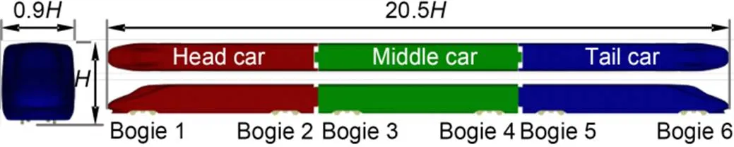
Fig. 1 Three-car grouped geometry model of CRH2

2.2 Numerical method

The IDDES with shear-stress transport (SST)turbulence model is used in ANSYS Fluent to investigate the temperature effect on the underbody flow characteristics beneath the HST. The introduction of the IDDES method has been described in previous publications (Menter, 1994; Shur et al., 2008; Ghasemian and Nejat, 2015). The governing equations were solved using the commercial finite-volume computational fluid dynamics (CFD) software. Simulations were performed using a pressure-based solver. The SIMPLE (semi-implicit method for pressure-linked equations) algorithm was used to update the pressure and velocity fields. The bounded central differencing scheme and the second-order upwind scheme were used to solve the momentum and theequations, respectively. The second-order implicit scheme was used for temporal advancement. The physical time step Δ=5×10-5s. The CFL number was less than 1.0 in more than 99% of the computational cells during the entire simulation, with a maximum value of 3.0 (Naung et al., 2021; Nakhchi et al., 2022).

2.3 Computational domain and boundary conditions

To correspond to the operation of the HST on the railway, the model of the HST is placed on a single-track ballast and rail (STBR) replica, which is 1/8th scaled. The model of the HST and the STBR are both placed in a computational domain to fit the flow field around the HST. The computational domain is shown in Fig. 2. The length of the domain is=65, and the width is=20. To make the blockage ratio of the computational domain less than 5% in the-axis direction, the height of the domain is=16. The distance between the front surface of the domain and the head of the car body is1=15, and the distance from the tail nose to the rear surface is2=29.5. For the IDDES simulation, the incoming flow speed applied at the inlet is 60 m/s. That is the same as the operating velocity of the HST on the high-speed railway and is defined as the velocity-inlet boundary condition on the front surface relative to the direction of the train operation. The rear surface is defined as the pressure-outlet and a zero static pressure is given. The side surface and top surface of the domain are defined as the symmetry. The lower surface with the STBR and the car body surface are defined as a no-slip wall. To investigate the influence of lower operating temperatures on the aerodynamic characteristics and the flow structures around the HST, four operating temperatures of +15 ℃, 0 ℃, -15 ℃, and -30 ℃ are selected. At +15 ℃, the Reynolds number in the IDDES simulation is=1.85×106based on the reference velocityrefand the reference heightof the HST.

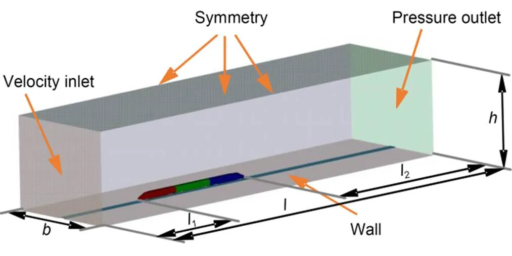
Fig. 2 Computational domain

2.4 Computational grid

A hexahedral dominated mesh is designed for numerical simulations. This type of mesh has been widely used for the numerical predictions of the flow characteristics around HSTs (Dong et al., 2019, 2020; Wang JB et al., 2019, 2020a, 2020b). Fifteen prism layers are used to accurately predict the turbulent boundary layer development along the surface of the HST, and the stretching ratio of the prism layers is set as 1.25, ensuring a good transition between the prism layers and the hexahedral mesh region, as described in Fig. 3. There is a refinement region of the mesh resolution beneath the HST. To fit the numerical method, the normalized resolution of the surface in the wall-normal direction+is less than 1.0.

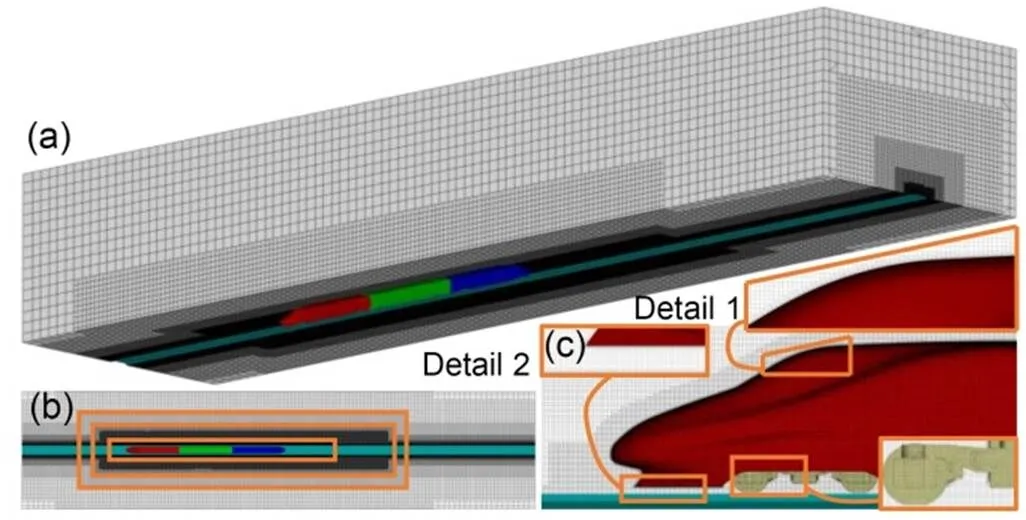
Fig. 3 Grid: (a) integral grid; (b) grid of the refinement region; (c) grid of prism layers

2.5 Numerical validation

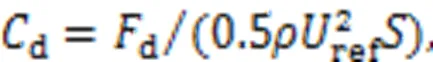
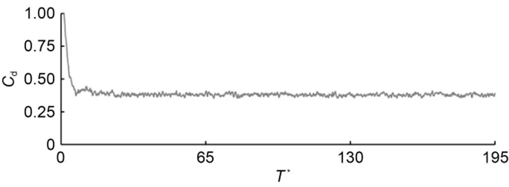
Fig. 4 Time history of the Cd value of the HST

From Fig. 4, it can be seen that with the rise of the computational time, the value of the aerodynamic drag coefficient is gradually convergent. To better describe the trend of the resistance with time, the time is dimensionless. We define*=ref/, whererefis 60 m/s. From the formulation, the time of the inlet-flow run through the computational domainround*=65, and the total computational timetotal*=195, which means the airflow runs three rounds inside the domain. From Fig. 4, the aerodynamic drag force coefficient of the HST airflow has converged at*=65, and the airflow has stabilized. Therefore, it is proved that the present grid can converge effectively and the computational results after*=65 can be adopted.

The same grid discretization method is used to re-discretize the computational domain, in which the size of the grid is scaled up and down by a ratio of 1.5 to obtain a coarse grid and a fine grid; the existing grid is defined as the middle grid. The coarse grid is 32 million, the middle grid is 59 million, and the fine grid is 98 million. The coarse grid and fine grid both converge well for the same time step by the same numerical calculation method. Time-averaged calculations were performed for numerical results in the range of*=65 to*=195 and compared to previous researchers' experimental results in an 8 m×6 m wind tunnel of the China Aerodynamics Research and Development Center (CARDC) (Zhang et al., 2018). In both the experiments and the numerical simulations an STBR model is placed at the bottom of the vehicle, with the ground and the STBR model as stationary walls. The temperature in the computational domain is kept at the same temperature as in the experiments. The aerodynamic forces are measured using a force measuring balance and the pressure values are measured using pressure sampling equipment. The blockage ratio in the test section of the wind tunnel was less than 1%. The results are listed in Table 1.

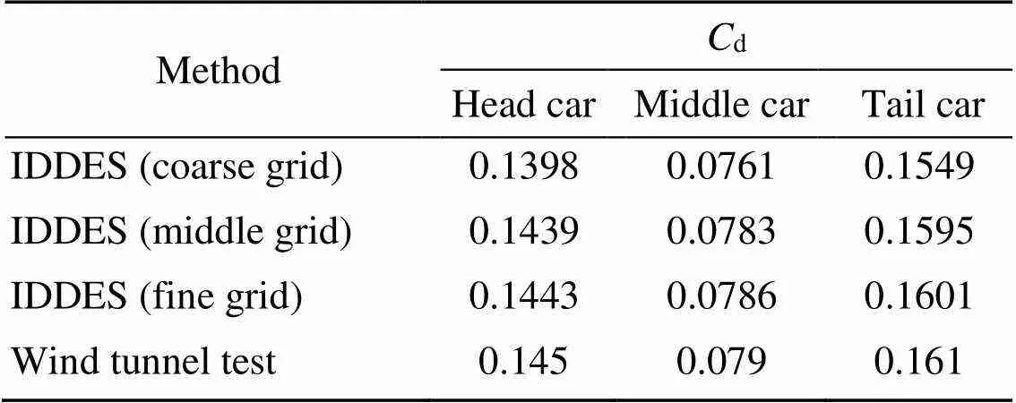
Table 1 Drag coefficients of each car for numerical result and wind tunnel test

Comparing the aerodynamic drag coefficients simulated by the IDDES method using different grids with the measured aerodynamic drag coefficients from the wind tunnel tests listed in Table 1, it can be found that the coarse grid, middle grid, and fine grid all have good aerodynamic calculation performance. For the coarse grid, the errors of the head, middle, and tail vehicles are less than 5%, while for the middle grid and fine grid, the errors of the head, middle, and tail vehicles are less than 1%, which indicates that for the middle grid and fine grid, the IDDES calculation method can simulate the aerodynamic characteristics of each vehicle very well. However, the computational resource consumption of the fine grid is too large, so in this study the middle grid is used for further calculations.

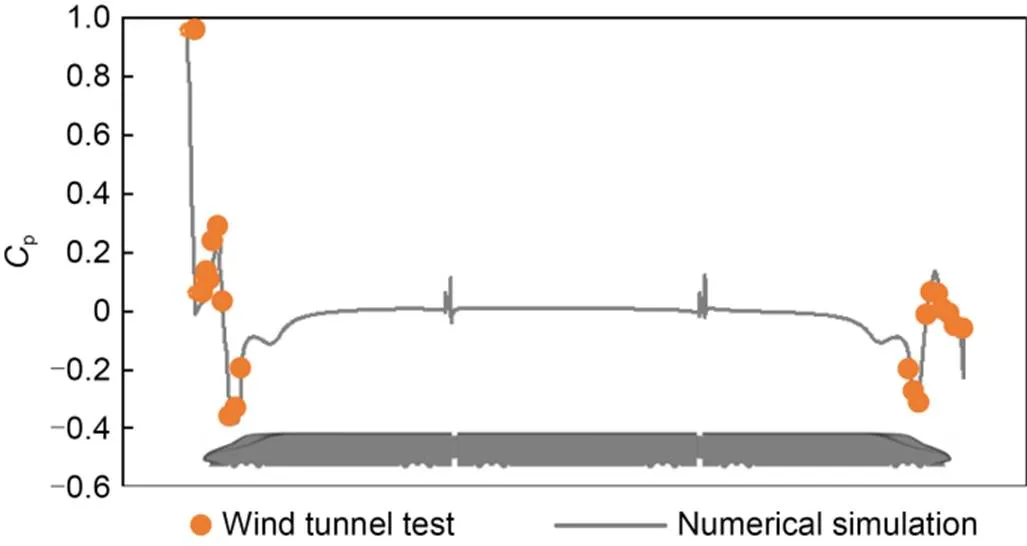
Fig. 5 Validation of the pressure on the surface of the HST

As can be seen in Fig. 5, the numerically calculated pressure values at the sampling line on the vehicle surface correspond well with the values at the measurement points at the same locations on the vehicle surface in the wind tunnel test. The pressure distribution on the train surface can, therefore, be effectively simulated by using the IDDES model in combination with the existing grid, so the results can be further analyzed.

3 Results and discussion

3.1 Aerodynamic drag force

The aerodynamic drag force is an important indicator of the aerodynamic performance of a train and its value is directly related to the changes in the flow field around the body. The smaller the aerodynamic drag force, the smaller the energy consumption of the train during operation. However, the flow field around the car body is directly related to the temperature of the airflow. The most intuitive effect of the change in environmental temperature on the train operation is reflected in the change in aerodynamic force. Thus, it is necessary to make a direct observation of the change in the aerodynamic drag force of the HST at different temperatures. To calculate and analyze the change of force more precisely, the car bodies of the head car, middle car, and tail car are divided into six parts respectively and, including six bogies, the whole car is divided into 24 parts, which are named hc1 to hc6, mc1 to mc6, tc1 to tc6, and bogie 1 to bogie 6, as shown in Fig. 6. The drag force of each part of the HST is shown in Fig. 7.

For a better analysis of the aerodynamic drag force of the HST, the train is divided into upper-part, lower-part, and bogie-part of the head car, middle car, and tail car. Figs. 7a–7d show the drag forces of each car of the HST, the upper-part, the lower-part, and the bogie-part, respectively. From Fig. 7, it can be found that as the temperature gradually decreases, there are certain changes in the forces on each part of the HST and the whole car body, and the aerodynamic drag of the whole car increases by 4.9% at 0 ℃, 10.9% at -15 ℃, and 16.9% at -30 ℃ compared to the aerodynamic drag of the HST operating at +15 ℃. In Fig. 7a, when the temperature decreases from +15 ℃ to -30 ℃, there is a rise in the aerodynamic drag force of the head car, middle car, and tail car of the HST. It can be found that for the aerodynamic drag of the head car, middle car, and tail car, the differences in the case of +15 ℃ and 0 ℃, the case of 0 ℃ and -15 ℃, and the case of -15 ℃ and -30 ℃ are all the same. Among these differences, the aerodynamic drag increases more for the head car and the tail car, and less for the middle car. The increments of aerodynamic drag of the head and tail cars are equal, while that for the middle car is less by approximately a half. In Fig. 7b, as the temperature decreases, the aerodynamic drag in the upper-part of the train increases to different degrees mainly concentrated in the parts named mc2, tc2, and tc6 and, with a similarly constant change in temperature, producing nearly the same numerical increase in drag. In Fig. 7c, the drag force increase is changed to the parts named hc1, hc5, mc1, mc5, tc1, and tc5. Fig. 7d shows the relationship between the aerodynamic drag force and the temperature on the bogie-part and shows that there is a significant drag rise only at the front-end bogie (bogie 1) of the HST.

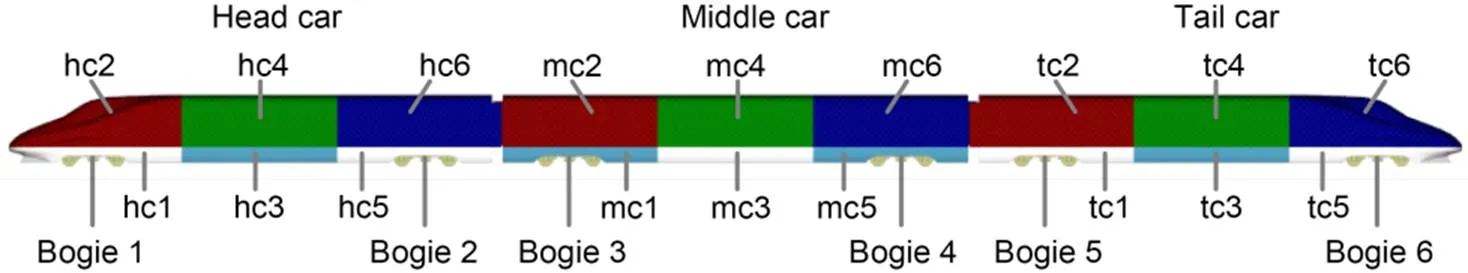
Fig. 6 Name of each part of the HST

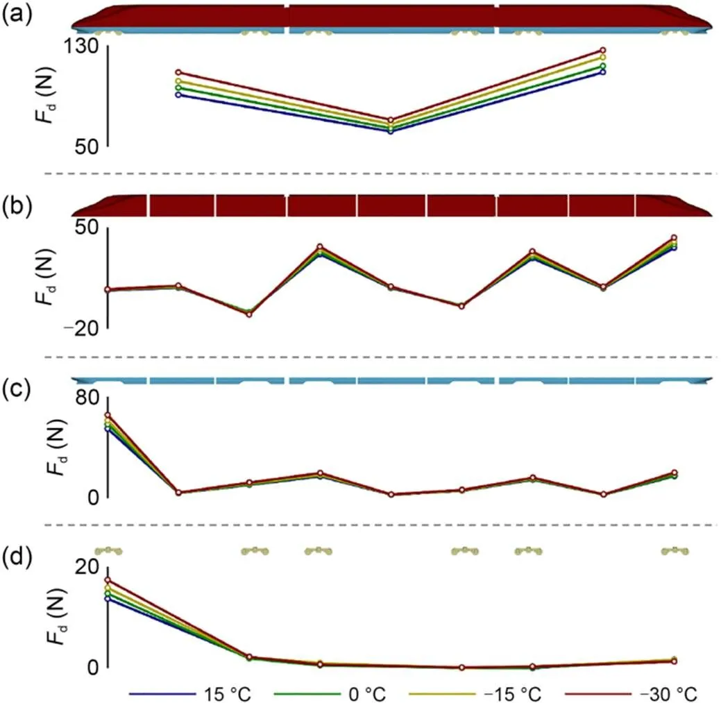
Fig. 7 Aerodynamic drag force of each part of the HST: (a) drag force of each car; (b) drag force of the upper-part; (c) drag force of the lower-part; (d) drag force of the bogie-part

From the variation of aerodynamic forces on the train with temperature, it can be seen that the lowering of temperature will cause a more serious aerodynamic drag increase for the train running on the open line, and the aerodynamic force reduction values between the different temperatures selected are almost equal as the temperature decreases, so the aerodynamic drag on the train at higher and lower temperatures can be roughly predicted. In addition, the changes in aerodynamic drag force in each part of the train are mainly concentrated in the upper-part of the train at mc2, tc2, and tc6, in the lower-part of the train at hc1, hc5, mc1, mc5, tc1, and tc5, and in bogie 1. These parts of the vehicle geometry represent either the surface flow separation phenomenon or the obvious impinging flow. Therefore, the influence of different operating temperatures on the aerodynamic drag force of the HST is chiefly reflected in the impingement and separation of the airflow on the surface.

Further analysis of the train aerodynamics is carried out. The change in aerodynamic drag due to temperature changes is mainly caused by the density and viscosity of the air and can be divided into two parts: the change in differential pressure drag and the change in viscous drag. Differential pressure drag will be described later. For the viscous drag variation, it has been found in previous studies that the viscous drag coefficient is proportional to the density-viscosity coupling coefficient (6/71/7) (Shi et al., 2021). When the temperature in the calculation domain around the train is reduced from +15 ℃ to -30 ℃, the air density increases by 18.6% and the air viscosity decreases by about 12.3%. According to the coupling coefficient calculations, there is still an increase in the coupling coefficient with decreasing temperature under the combined effect of the changes in air density and viscosity. This indicates that there is an increase in viscous drag at lower temperatures, which in turn leads to an increase in the aerodynamic drag of the train. A test of the viscous drag component of the aerodynamic drag of the total HST shows that when the temperature is reduced from +15 ℃ to -30 ℃, the viscous drag rises by approximately 13.67%, which is in good agreement with the 13.59% increase in the density-viscosity coupling coefficient, further demonstrating that the change in aerodynamic drag of HST at low temperatures is directly related to air density and viscosity.

3.2 Pressure distribution

As another effect of the impinging flow variation acting on the body surface, the variation of the pressure distribution on the HST body surface at different temperatures is investigated. Fig. 8 shows the time-averaged pressure distribution near the train at the middle section in the-axis direction. Figs. 8a‍–‍8d show the pressure distribution of the train at +15 ℃, 0 ℃, -‍15 ℃, and -‍30 ℃ and the pressure contours are equal to +200 Pa and -200 Pa, respectively, where the positive pressure contours are marked in red and the negative pressure contours are marked in blue. Fig. 8e extracts the pressure contours from the above images and fixes them in the same coordinates for comparison of the contour distribution locations. It can be found that in the middle section in the-axis direction, the pressure distribution trends around the train are similar, although the ambient temperature is different. However, in contrast, as the temperature decreases, there is a gradual increase in both the positive and negative pressure zones on the mid-section, and they are mainly concentrated in the head area of the head car and the tail area of the tail car. The variation of pressure with temperature is well demonstrated in Fig. 8e. As the temperature gradually decreases, it can be found that the positive pressure contours at the nose of the head car and the negative pressure contours at the top of the car body both produce a significant outward expansion phenomenon. Similarly, the positive pressure contours on the surface of the nose and near the flow field distribution of the tail car and the negative pressure contours at the top of the tail car show outward expansion. It can be seen that the ambient temperature affects the pressure distribution in the flow field around the train, in which the higher the temperature the smaller the diffusion area of the positive and negative pressure distribution near the car body, and the lower the temperature the larger the diffusion area of the positive and negative pressure distribution near the car body. In addition, there is a direct relationship between the pressure on the surface of the car body and the air density. The enhancement of pressure with decreasing temperature further indicates that the increase in air density due to temperature is the underlying reason for the increase in the differential pressure drag component of the aerodynamic drag.

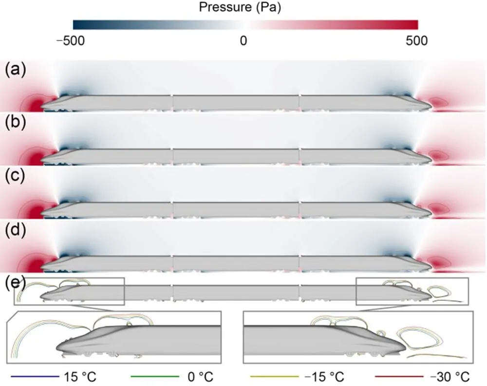
Fig. 8 Pressure distribution at the mid-section in the y-axis: (a) +15 ℃; (b) 0 ℃; (c) -15 ℃; (d) -30 ℃; (e) comparison of the pressure contour distribution

However, it can be found that although Fig. 8 can effectively reflect the trend of pressure distribution in the flow field domain near the car body at different temperatures and the differences in the pressure region in the cases at different temperatures, the marked areas are mainly concentrated in the upper region of the car body. The lower region of the flow field, especially the region inside the bogie cavities, cannot be clearly shown in the cross section. Therefore, the sampling line of the lower-part of the car body regarding the pressure value is made at the mid-section of the HST in the-axis direction and the results are shown in Fig. 9. The position of the sampling line is shown as the orange line in the figure.

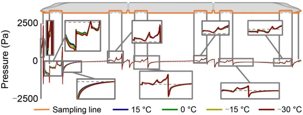
Fig. 9 Pressure value at sampling line of the HST

From Fig. 9, it can be found that the trend of pressure distribution at the bottom of the car body is basically the same at different temperatures, and the fluctuations and differences in pressure values are mainly reflected in the bogie cavities of the body and its nearby areas. From the pressure distribution details of each bogie cavity and its nearby areas it can be found that the most obvious pressure variation with temperature exists at the cavity of bogie 1. From the detailed figure, it can be found that the flow field at the cavity of bogie 1 and nearby mainly distributes negative pressure downstream. With the gradual decrease of temperature, the negative pressure value of the surface near the cavity gradually increases and gets its maximum value at -‍30 ℃. The cavity from bogie 2 to bogie 5 mainly distributes positive pressure. As the temperature gradually decreases, the positive pressure value in the cavity gradually increases. Similarly, the positive pressure in the bogie cavity reaches its maximum value at -30 ℃. The cavity of bogie 6 has both positive and negative pressure zones, and it can be found from the detailed figures that both positive and negative pressures increase as the temperature decreases and still reach their maximum value at -‍30 ℃. In summary, the temperature decrease will have a certain increased effect on the pressure values of both positive and negative pressure zones on the surface of the bottom of the HST.

To further investigate the effect of temperature changes on the pressure distribution on the body surface of the lower region of the HST, especially the effect of temperature-influenced impinging flow acting on the geometrically complex bogie cavity areas at the bottom of the vehicle, the pressure distribution at the bottom of the car body is shown in Fig. 10. Figs. 10a–10d show the pressure distribution at the bottom of the car body at temperatures of +15 ℃, 0 ℃, -‍15 ℃, and -‍30 ℃, respectively, where rectangles 1 to 5 are marked to show the changes of pressure distribution in the bogie cavities due to temperature.

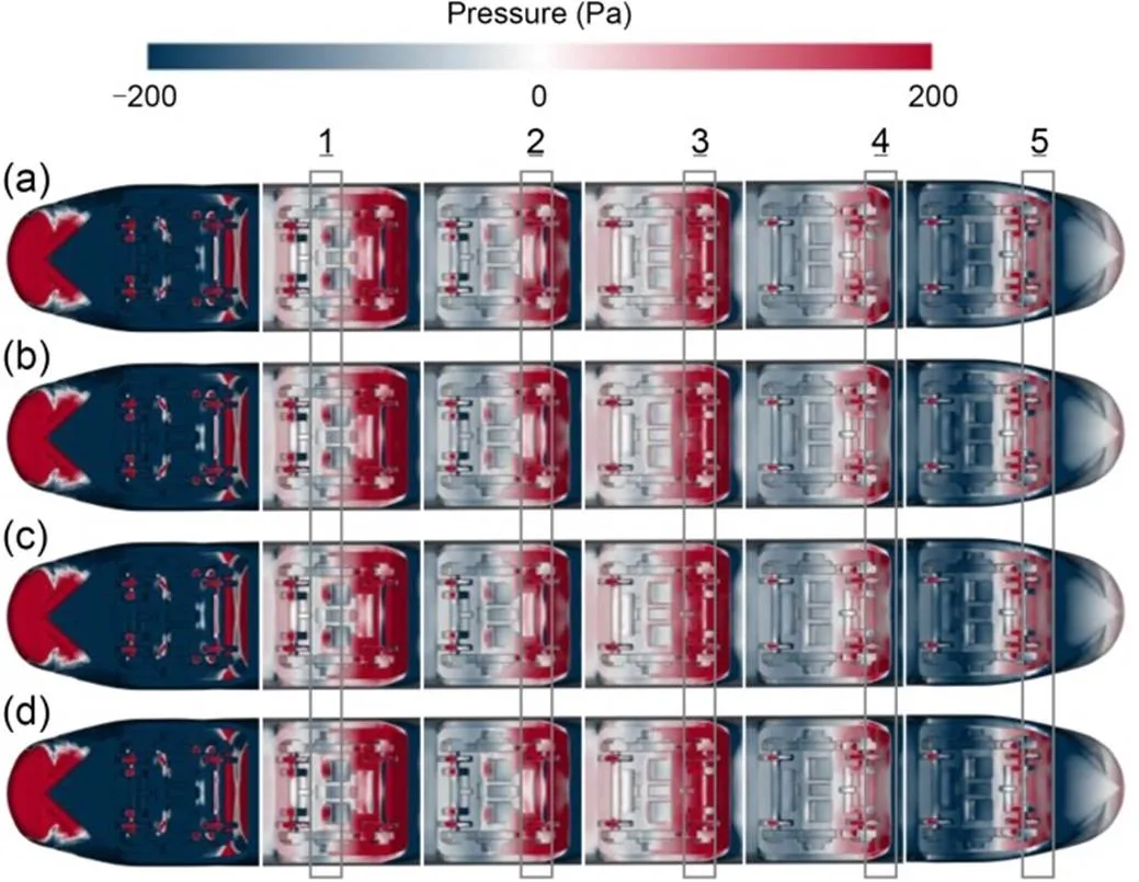
Fig. 10 Pressure distribution at the bottom of the HST: (a) +15 ℃; (b) 0 ℃; (c) -15 ℃; (d) -30 ℃

In rectangle 1 it can be found that at the center of the bogie, on the windward side of the structure subject to the impinging flow, the pressure distribution area in the positive pressure zone gradually increases as the temperature decreases and the pressure values in its positive pressure zone are enhanced. The strongest positive pressure distribution is obtained at -‍30 ℃. Similarly, the growth of positive pressure zone distribution with decreasing temperature exists at rectangle 2 as well as rectangle 3, which represents the position of the bogie rear-wheelset axle and is accompanied by an increase of positive pressure intensity. The enhancement of the positive pressure zone with decreasing temperature is more pronounced in rectangles 4 and 5, representing the position of the rear end plate of the bogie cavities. Meanwhile, the analysis of the pressure distribution in the cavity of bogie 6 reveals that there is a significant negative pressure zone in the front area of the cavity. As the temperature decreases, the distribution range and negative pressure intensity of this negative pressure zone are significantly higher. The pressure variation of the positive and negative pressure zones with temperature further demonstrates that a decrease in temperature affects the pressure distribution of the vehicle surface, especially the windward area. In the low-temperature environment, there will be more severe positive and negative pressure distribution in both the upper-part and lower-part of the car body, as well as the bogie-part, and the lower temperature will contribute to stronger impacts on the bogie and rear panels of the cavity, which will reduce the aerodynamic characteristics of the HST during regular operation.

Fig. 11 shows the time-averaged pressure values along the streamwise sampling lines beneath the HST. The streamwise sampling linesl1,l2, andl3are located in the mid-section of the-axis direction with the heights of the top of subgrade which are defined as=0.086,=0.130as the top of the rails, and=0.173as the trackside height proposed by Technical Specification for Interoperability (TSI) (CEN, 2013); the results are presented in Figs. 11a–11c respectively. Generally, the time-averaged pressure value increases sharply as the cowcatcher of the head car passes by. After that, it decreases rapidly due to the acceleration effect of the cowcatcher on the local airflow. Then, the second sharp peak of time-averaged pressure occurs near the tail car but the peak-to-peak value beneath the head car is far larger than that beneath the tail car. As can be seen in Fig. 11, the pressure values at the different sampling lines are all consistent with those mentioned above. Comparing the pressure values at the three sampling lines separately, it can be found that the increases in pressure values at the cowcatcher part of the head car, Figs. 11a–11c, are all affected by the temperature. As with the previous conclusions obtained about the pressure, the positive pressure values located at the cowcatcher of the head car are greater as the temperature decreases, and the positive pressure at the cowcatcher has its maximum value when the temperature reaches -30 ℃. At the location of the cavity of bogie 1 downstream of the cowcatcher, the temperature decrease has an effect on the distribution of the negative pressure zone there, where the pressure value in the negative pressure zone is the least at a temperature of +15 ℃ and the greatest at -30 ℃. In addition, in the peak-to-peak value of the pressure at the sampling lines beneath the HST, it is possible to conclude that the lower the temperature the larger the value and the higher the temperature the smaller the value.

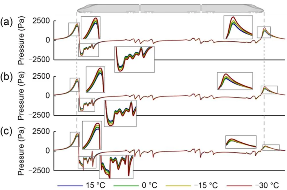
Fig. 11 Pressure values along the sampling lines beneath the HST: (a) lx1; (b) lx2; (c) lx3

Similarly, the effect of temperature on the pressure variation of the flow field at the bottom of the train exists at the cowcatcher of the tail car. From Fig. 11, it can be found that at linel1, the magnitude of its pressure fluctuation is larger and therefore the effect of temperature on pressure variation is greater, while at linesl2andl3, the magnitude of pressure variation is smaller and therefore the effect of temperature on pressure variation is smaller. But still, the maximum value is obtained at the lowest temperature and the minimum value at the highest temperature. Meanwhile, the maximum peak-to-peak pressure variation is still at a temperature of -30 ℃ and the minimum value is at +15 ℃ at the tail car. Therefore, lower operating temperatures will lead to stronger pressure fluctuations in the flow field between the bottom of the car and the surface of the STBR, which in turn will reduce the aerodynamic performance of the bottom of the car, for example leading to more snow particles suspended in the flow area under the car and thus more severe snow accumulation in the bogie area (Zhu and Hu, 2017; Jing et al., 2019).

3.3 Flow round the HST

Fig. 12 shows the contour surface of the train-induced wind velocity in the flow field around the vehicle and the contour lines at different height sections. The train-induced wind coefficient*‍=/refis defined, whereis the wind velocity formed in the flow field around the vehicle by the train operation. Fig. 12a shows the coefficient contours at +15 ℃, 0 ℃, -15 ℃, and -30 ℃ colored asω, vorticity values on the-axis. Fig. 12b shows the train-induced wind coefficient*=0.1 at 0.38implying the height of the equipment on the platform inside the station, and Fig. 12c shows the train-induced wind coefficient*=0.1 at 0.05implying the height of the equipment beside the track. From Fig. 12a, it can be found that the distribution regions of the contour surface of the train-induced wind around the car have approximately the same shape, mainly at the head of the head car, near the perimeter of the HST, and at the downstream flow field of the tail car. The distribution of the vortex volume on the contour surface is the same. The distribution of the train-induced wind contour lines around the vehicles at different temperatures in Fig. 12b is the same, which means that the influence of the train-induced wind on the equipment on the platform in the station at different temperatures does not change much. The distribution of contour lines in Fig. 12c has some differences and is mainly concentrated in the flow field at the rear area of the tail car, while the contour positions at the head of the head car and the side of the HST do not change much. To better analyze the variation of contour positions in the tail flow field of the tail car, a detailed figure of the contours in the tail flow field in Fig. 12c is made and the contours at the temperature of +15 ℃ and -30 ℃ are screened for a clearer comparison. It can be found that as the temperature decreases, the contour line from the front of the tail car produces a contraction toward the car body, but to a lesser extent. As the airflow extends downstream towards the vehicle, the inward contraction of the contours gradually increases, and the maximum distance between contours is obtained at the wake. It can be seen that the decrease in temperature reduces the intensity of the train-induced wind around the vehicle, leading to an inward contraction of the train-induced wind action and reducing the impact of the wind on the trackside equipment.

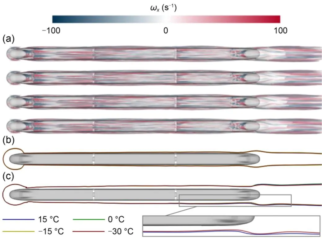
Fig. 12 Contour surfaces and lines of U* around the car body: (a) contour surfaces of U*; (b) contour lines of U* at the height of 0.38H; (c) contour lines of U* at the height of 0.05H

To further investigate the variation of the flow field around the train at high and low temperatures, the vorticity value of the surrounding airflow in the-axis of the HST which is defined asωis shown in Fig. 13, where the height of the section is located at 0.27. To show more clearly the effect of high and low temperatures on the flow field near the car, only the images at +15 ℃ and -30 ℃ are shown in Fig. 13. Fig. 13a shows the vortex cloud at +15 ℃, Fig. 13b shows the vortex cloud at -30 ℃, and Fig. 13c shows the comparison of the contours of positive and negative vorticity values of 50 at the two temperatures, respectively. From Fig. 13, it can be found that the vorticity distribution around the car body is the same at different temperatures. On one side of the car body, a positive vorticity region is generated from the head of the head car and continues and develops toward the tail, and on the other side, a negative vorticity region continues and develops toward the tail as well, and two vorticity regions are derived from the nose of the tail car in the opposite direction of the corresponding side. However, further analysis of the vorticity contours shows that the distribution of the zones at the nose of the tail car is similar at different temperatures, and the extension distance to the downstream flow field is the same, but the vorticity contours at the head of the car and extending to the tail have some differences. It can be seen that the decrease in temperature will significantly enhance the vorticity contained in the-axis of the vortex flow generated on both sides of the head car and prolong the distance of vorticity development to the downstream flow field, which will have a more serious impact on the wake flow at the tail of the HST.

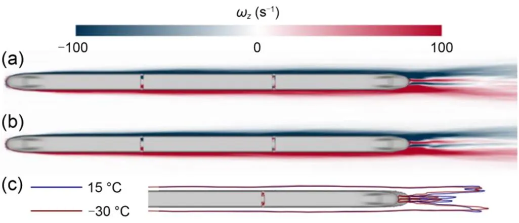
Fig. 13 ωz value around the HST of the section at 0.27H height: (a) +15 ℃; (b) -30 ℃; (c) comparison of the contours of positive and negative vorticity values

The airflow at the bottom of the car body needs further analysis. The train-induced wind coefficients*at the bottom of the train were sampled at sampling linesl1,l2, andl3, respectively, and the sampling results are shown in Fig. 14, where Figs. 14a–14c show the results forl1tol3, respectively. Generally, the underbody airflow velocity increases along the streamwise direction, owing to the increasing boundary layer thickness, and the maximum underbody slipstream velocity appears in the vicinity of the cowcatcher of the tail car. As can be found in Fig. 14, the coefficients at each sampling line have basically the same variation pattern. A detailed diagram of several key parts of the sampling line, such as the nose of the head car, the connection in the middle of the vehicle, and the bogie and cowcatcher of the tail car, shows that there is a significant effect of temperature change on the airflow velocity at the bottom of the train. It is found that, as the temperature gradually decreases, the velocity coefficient at the sampling line has a significant increase and is mainly concentrated in the critical area, indicating that the operating temperature will have a dominant effect on the air flow below the HST. At the same time, it can be found that the key area is mostly the geometrically unsmooth area at the bottom of the car body, while in the geometrically smooth area, such as the bottom of the equipment cavities of the car body, there is no significant change in velocity with temperature, which shows that the influence of temperature on the train-induced wind velocity at the bottom of the car body is still mainly concentrated in the geometrically unsmooth area where the impinging flow is easily generated. Comparing the changes with temperature at different sampling lines, it can be found that as the sampling linesl1tol3gradually approach the car body, the sampling value of train-induced wind speed with temperature gradually decreases. It can be seen that the influence of temperature on the airflow around the train is mainly in the peripheral action area where the impinging flow is easily formed on the surface of the car body. In the vicinity of the impinging flow region, there are obvious fluctuations in the flow velocity around the vehicle, and the fluctuations in the flow velocity with temperature basically disappear.

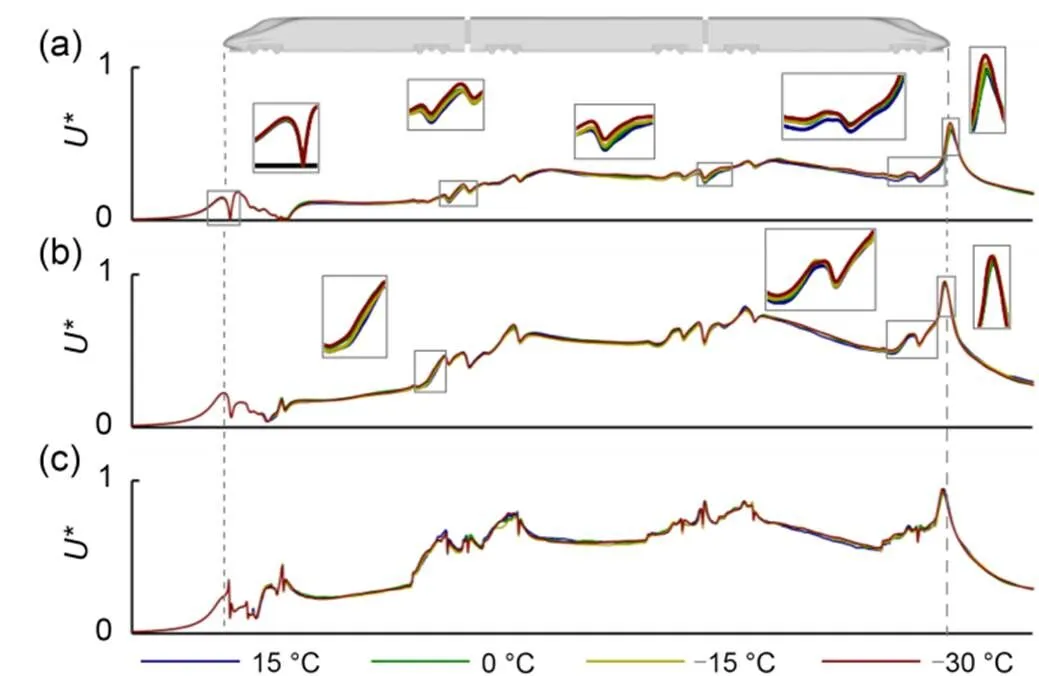
Fig. 14 U* value at sampling lines: (a) lx1; (b) lx2; (c) lx3

To further analyze the effect of the unsmooth parts of the bottom structure of the vehicle on the bottom airflow, the flow velocity of the airflow, defined as, was sampled at the regions near the rear plate of the cavities of bogies 2–5 located at the center of the vehicle; the results are shown in Fig. 15. Bogie cavities 1 and 6 were not selected to avoid the interference of the separated flow from the upper-part of the vehicle body at the nose to the airflow at the lower region of the car body. The sampling line is located at the middle section of the-axis of the HST, 0.5from the center plane of each bogie cavity, at a height from the root of the STBR to the upper surface of the cavity, whose position will be shown by the orange line in the figure. To clearly show the variation of airflow at different temperatures, only the images of +15 ℃ and -30 ℃ are still retained. From the figure, it can be seen that the air flow velocity in the cavity of bogie 2 and bogie 3 has increased when the temperature decreases from +15 ℃ to -30 ℃. Among them, cavity 2 is located at the relatively more upstream position, so the change of flow velocity is relatively more obvious. As the sampling coordinates move down and gradually away from the car body, the velocity values due to the temperature change increase. As it gradually approaches the bottom of the STBR, the velocity difference gradually decreases and is almost equal at the ground. At the cavities of bogie 4 and bogie 5, the change in flow velocity with temperature is relatively small because of their location further downstream, but there is still an increase in flow velocity as the temperature decreases. It can be seen that in the unsmooth region of the structure, where the impinging flow is easily formed, the airflow velocity is continuously affected by the temperature and does not disappear until near the ground, and the temperature change has a more obvious effect on the airflow velocity acting upstream compared to downstream.

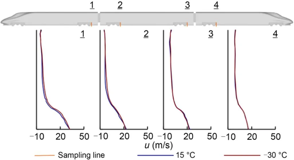
Fig. 15 Flow velocity at the sampling lines near the rear plate of the cavities of bogies 2–5

3.4 Wake flow

In the analysis of the flow field around the car body, it can be found that there is a significant change in the characteristics of the wake flow at different temperatures, so further analysis was conducted for the wake flow of the HST. Firstly, the train-induced wind at the tail of the car body was analyzed, and the results are shown in Fig. 16. The sampling lines are the orange lines in the figure, which are located at 0.05height and 0.38height, respectively, and the same distance of 0.81away from the-axis center of the vehicle. Fig. 16a shows the sampling results at 0.05, and Fig. 16b shows the sampling results at 0.38. By comparing the results for the temperatures of +15 ℃ and -30 ℃, it can be found that as the temperature decreases, there is a significant decrease in the train-induced wind coefficient at 0.05, while there is almost no change at 0.38. It can be seen that the temperature decreases the velocity of the train-induced wind around the car body and is mainly concentrated in the lower region of the vehicle, which is in good agreement with the results above for the train-induced wind in the wake flow.

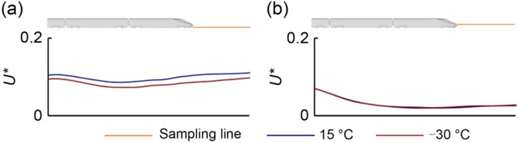
Fig. 16 Velocity of the train-induced wind at the wake flow of the HST: (a) sampling line at 0.05H height; (b) sampling line at 0.38H height

Fig. 17 shows the streamlines of the section of the flow field at the tail of the HST at distances of 1and 2from the car body and shows the distribution of vortices in the-axis and the location of the core of the vortex in the section. Among them, Fig. 17a shows the cases of the sections located atand 2when the temperature is +15 ℃, and Fig. 17b shows the cases of the sections located atand 2when the temperature is -30 ℃. Since the formation and development of the flow field around the HST have a certain symmetry, the analysis is performed on one side of the vehicle. From the figure, it can be seen that the sections at different locations at the rear of the vehicle have similar flow field structures at different temperatures and the trend of development downstream to the vehicle is the same. However, as the temperature decreases, there is an enhancement ofωat the section. At the same time, it can be found that the vortex at the bottom of the car body has a tendency to expand outward as the temperature decreases, which is mainly reflected in the outward change of the marked point of the core of the vortex in the figure. There are changes at the section at the distances ofand 2, and the vortex core moves farther at the section of 2. It can be seen that the lower temperature will cause the vorticity in the wake flow of the train to increase along the direction of train operation, and the outward movement of the vortex and the core indicates that there will be more obvious vortex structures and shedding in the wake region of the HST, implying that there will be a more extensive vortex influence zone and more serious vortex influence in the tail of the HST at a lower temperature.

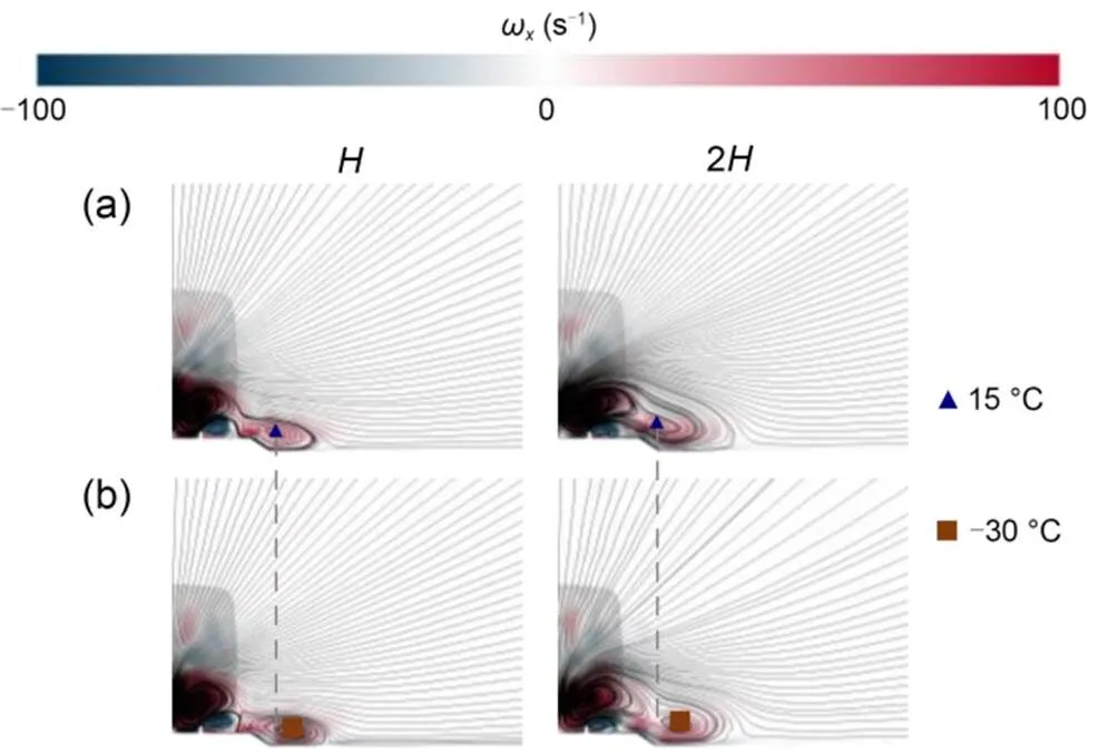
Fig. 17 Distribution of vortices at the section of the tail and the location of the vortex core: (a) +15 ℃; (b) -30 ℃

The airflow velocities at, 2, 4, and 6behind the car body are shown in Fig. 18, and the flow coefficient is defined as*=ref. The flow coefficient can well reflect the airflow in the rear region of the car body on the stationary ground during the actual operation of the HST. The height of the sampling line is located at a height of 0.27representing the farthest end at the nose of the tail car, and the width range is from the mid-plane in the-axis of the vehicle to the distanceaway. The sampling lines are defined as 1, 2, 3, and 4 and are shown as orange lines in the figure. A comparison of the results for +15 ℃ and -30 ℃ at the corresponding lines shows that on the left side of the grey dashed line, in the area directly behind the vehicle body and as the temperature decreases, the flow coefficient decreases near the center of the vehicle but gradually increases as it moves toward the outside of the car body and decreases slightly away from the area directly behind the HST. In the region away from the rear of the car body, the flow coefficients are equal between different temperatures. This pattern is well found at line 2 as well, but the velocity coefficients are already essentially equal at the boundary of the region directly behind the car body. At line 3, the variation of the velocity coefficient is still present but significantly reduced, and at line 4 there is no variation of the velocity coefficient. At the same time, it is obvious that the location of the peak value is farther away from the center of the car body as the temperature decreases at lines 1 and 2, which further indicates the existence of vortex outward expansion of the wake flow.

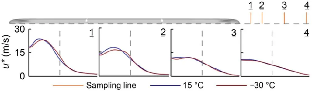
Fig. 18 Comparison of flow velocity coefficients at the y-axis sampling lines

The results at the-axis sampling lines at the rear of the car body are shown in Fig. 19, where the sampling lines 1, 2, 3, and 4 are located far from the car body at, 2, 4, and 6, respectively, in the mid-plane of the-axis of the car body; their height is 1.5. From Fig. 19, it can be found that as the temperature decreases, the affected area of the velocity coefficient*is mainly concentrated in the lower region of the car body near the STBR and decreases significantly, while in the upper region it does not vary much. This further proves that the influence of temperature on the velocity of the wake flow of the HST is mainly concentrated in the bottom of the car body and implies that the decrease in temperature causes the HST to have a relatively weaker effect on the equipment on both sides of the track.

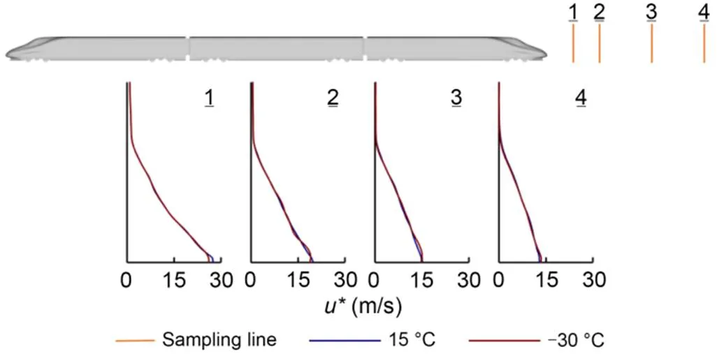
Fig. 19 Comparison of flow velocity coefficients at the z-axis sampling lines

4 Conclusions

In this study, an IDDES method based on the SSTturbulence model has been used to investigate the underbody flow characteristics beneath an HST operating at lower temperatures with=1.85×106. The accuracy of the numerical method has been validated by wind tunnel experiments and full-scale tests. The results are summarized as follows.

The temperature has an effect on the operating drag force of the HST. Compared to the normal temperature of +15 ℃, the operating resistance of the HST at low temperatures increases by 4.9% (0 ℃), 10.9% (-15 ℃), and 16.9% (-30 ℃), respectively, mainly in hc1, hc5, and bogie 1 of the head car, mc1, mc2, and mc5 of the middle car, and tc1, tc2, tc5, and tc6 of the tail car. The effect of temperature on the aerodynamic drag of HST is more serious than on the impingement and separation of surface flow.

As the temperature decreases, both the positive and negative pressure zones in the upper body region expand significantly, and the peak value under the body increases significantly. In the bogie cavities, the windward side of the bogie, which is susceptible to airflow impact, and the rear end plate of the cavity show a significant increase in positive pressure. The pressure distribution of the flow field under the car body shows an obvious increase, and is mainly concentrated in the nose of the head car and the cowcatcher of the tail car.

As the temperature decreases, the range of train-induced wind action around the body is significantly reduced, and the distribution area of the vorticity at the nose of the tail car produces a significant backward extension. In the lower-part, the velocity of train-induced wind increased significantly with the temperature reduction and was mainly concentrated in the area susceptible to impingement flow. The airflow velocity in the bogie cavities increased significantly and was mainly concentrated in the upstream cavities.

The wake flow of HST is affected by temperature mainly in the near region of the downstream flow field of the car body and the bottom of the wake flow. As the temperature decreases, there is a significant decrease in the train-induced wind at the bottom of the wake flow, while there is little difference at the top. The vortex generated at the rear of the tail car expands outwards significantly, and the vorticity increases significantly too.

This work is supported by the National Natural Science Foundation of China (Nos. 52172363 and 52202429), the National Key Research and Development Program of China (No. 2020YFF0304103-03), and the Independent Exploration of Graduate Students of Central South University (No. 2019zzts268), China.

Guangjun GAO designed the research. Jiabin WANG and Yan ZHANG processed the corresponding data. Xiujuan MIAO wrote the first draft of the manuscript. Wenfei SHANG helped to organize the manuscript. Xiujuan MIAO and Wenfei SHANG revised and edited the final version.

Xiujuan MIAO, Guangjun GAO, Jiabin WANG, Yan ZHANG, and Wenfei SHANG declare that they have no conflict of interest.

CEN (European Committee for Standardization), 2013. Railway Applications—Aerodynamics. Part 4: Requirements and Test Procedures for Aerodynamics on Open Track, EN 14067-4:2013. CEN.

Dong TY, Liang XF, Krajnović S, et al., 2019. Effects of simplifying train bogies on surrounding flow and aerodynamic forces., 191:170-182. https://doi.org/10.1016/j.jweia.2019.06.006

Dong TY, Minelli G, Wang JB, et al., 2020. The effect of ground clearance on the aerodynamics of a generic high-speed train., 95:102990. https://doi.org/10.1016/j.jfluidstructs.2020.102990

Dorigatti F, Sterling M, Baker CJ, et al., 2015. Crosswind effects on the stability of a model passenger train—a comparison of static and moving experiments., 138:36-51. https://doi.org/10.1016/j.jweia.2014.11.009

Fujii T, Kawashima K, Iikura S, et al., 2002. Preventive measures against snow for high-speed train operation in Japan. The 11th International Conference on Cold Regions Engineering, p.448-459. https://doi.org/10.1061/40621(254)38

Gao GJ, Zhang Y, Xie F, et al., 2019. Numerical study on the anti-snow performance of deflectors in the bogie region of a high-speed train using the discrete phase model., 233(2):‍141-159. https://doi.org/10.1177/0954409718785290

Gao GJ, Zhang Y, Wang JB, 2020. Numerical and experimental investigation on snow accumulation on bogies of high-speed trains., 27:1039-1053. https://doi.org/10.1007/s11771-020-4350-x

Ghasemian M, Nejat A, 2015. Aerodynamic noise prediction of a horizontal axis wind turbine using improved delayed detached eddy simulation and acoustic analogy., 99:210-220. https://doi.org/10.1016/j.enconman.2015.04.011

Han YD, Chen DW, Liu SQ, et al., 2020. An investigation into the effects of the Reynolds number on high-speed trains using a low temperature wind tunnel test facility., 16(1):1-19. https://doi.org/10.32604/fdmp.2020.06525

Huang ZW, Feng YH, Gao GJ, et al., 2017. Numerical research of the snow and ice accumulation on the brake calipers of the high-speed trains., 14(12):2516-2524 (in Chinese). https://doi.org/10.3969/j.issn.1672-7029.2017.12.002

Jing GQ, Ding D, Liu X, 2019. High-speed railway ballast flight mechanism analysis and risk management–a literature review., 223:629-642. https://doi.org/10.1016/j.conbuildmat.2019.06.194

Jing JE, Gao GJ, 2013. Simulation of the action effect of wind-driven rain on high-speed train., 10(3):99-102 (in Chinese). https://doi.org/10.19713/j.cnki.43-1423/u.2013.03.020

Kloow L, 2011. High-Speed Train Operation in Winter Climate. KTH Railway Group Publication, Stockholm, Sweden.

Liu MY, Wang JB, Zhu HF, et al., 2019. A numerical study of snow accumulation on the bogies of high-speed trains based on coupling improved delayed detached eddy simulation and discrete phase model., 233(7):715-730. https://doi.org/10.1177/0954409718805817

Men JQ, 2015. Dynamic Performance Investigation of Alpine EMU at Low Temperature Conditions. MS Thesis, Southwest Jiaotong University, Chengdu, China (in Chinese).

Menter FR, 1994. Two-equation eddy-viscosity turbulence models for engineering applications., 32(8):1598-1605. https://doi.org/10.2514/3.12149

Nakhchi ME, Naung SW, Dala L, et al., 2022. Direct numerical simulations of aerodynamic performance of wind turbine aerofoil by considering the blades active vibrations., 191:669-684. https://doi.org/10.1016/j.renene.2022.04.052

Naung SW, Nakhchi ME, Rahmati M, 2021. Prediction of flutter effects on transient flow structure and aeroelasticity of low-pressure turbine cascade using direct numerical simulations., 119:107151. https://doi.org/10.1016/j.ast.2021.107151

Niu JQ, Sui Y, Yu QJ, et al., 2019. Numerical study on the impact of Mach number on the coupling effect of aerodynamic heating and aerodynamic pressure caused by a tube train., 190:100-111. https://doi.org/10.1016/j.jweia.2019.04.001

Raghunathan RS, Kim HD, Setoguchi T, 2002. Aerodynamics of high-speed railway train., 38(6-7):469-514. https://doi.org/10.1016/S0376-0421(02)00029-5

Rashidi MM, Hajipour A, Li T, et al., 2019. A review of recent studies on simulations for flow around high-speed trains., 5(2):311-333. https://doi.org/10.22055/JACM.2018.25495.1272

Shi JW, Li MX, Zhang SM, et al., 2021. Effect of low temperature on aerodynamic performance of pantograph., 57(2):190-199 (in Chinese). https://doi.org/10.3901/JME.2021.02.190

Shur ML, Spalart PR, Strelets MK, et al., 2008. A hybrid RANS-LES approach with delayed-DES and wall-modelled LES capabilities., 29(6):1638-1649. https://doi.org/10.1016/j.ijheatfluidflow.2008.07.001

Sui Y, Niu JQ, Ricco P, et al., 2021. Impact of vacuum degree on the aerodynamics of a high-speed train capsule running in a tube., 88:108752. https://doi.org/10.1016/j.ijheatfluidflow.2020.108752

Tai BW, Liu JK, Wang TF, et al., 2017. Numerical modelling of anti-frost heave measures of high-speed railway subgrade in cold regions., 141:28-35. https://doi.org/10.1016/j.coldregions.2017.05.009

Teng WX, 2019. Study on Dynamic Performance of High-Speed Trains at Low Temperature Environment. PhD Thesis, Southwest Jiaotong University, Chengdu, China (in Chinese). https://doi.org/10.27414/d.cnki.gxnju.2019.002176

Tian HQ, 2019. Review of research on high-speed railway aerodynamics in China., 1(1):1-21. https://doi.org/10.1093/tse/tdz014

Wang JB, Zhang J, Zhang Y, et al., 2018a. Impact of bogie cavity shapes and operational environment on snow accumulating on the bogies of high-speed trains., 176:211-224. https://doi.org/10.1016/j.jweia.2018.03.027

Wang JB, Gao GJ, Liu MY, et al., 2018b. Numerical study of snow accumulation on the bogies of a high-speed train using URANS coupled with discrete phase model., 183:295-314. https://doi.org/10.1016/j.jweia.2018.11.003

Wang JB, Minelli G, Dong TY, et al., 2019. The effect of bogie fairings on the slipstream and wake flow of a high-speed train. An IDDES study, 191:183-202. https://doi.org/10.1016/j.jweia.2019.06.010

Wang JB, Minelli G, Dong TY, et al., 2020a. An IDDES investigation of Jacobs bogie effects on the slipstream and wake flow of a high-speed train., 202:104233. https://doi.org/10.1016/j.jweia.2020.104233

Wang JB, Minelli G, Zhang Y, et al., 2020b. An improved delayed detached eddy simulation study of the bogie cavity length effects on the aerodynamic performance of a high-speed train., 234(12):2386-2401. https://doi.org/10.1177/0954406220907631

Wang JY, Wang TT, Yang MZ, et al., 2021. Effect of localized high temperature on the aerodynamic performance of a high-speed train passing through a tunnel., 208:104444. https://doi.org/10.1016/j.jweia.2020.104444

Wang WL, Liang YW, Zhang WH, et al., 2020. Experimental research into the low-temperature characteristics of a hydraulic damper and the effect on the dynamics of the pantograph of a high-speed train running in extreme cold weather conditions., 234(8):896-907. https://doi.org/10.1177/0954409719879029

Xie F, Zhang J, Gao G, et al., 2017. Study of snow accumulation on a high-speed train’s bogies based on the discrete phase model., 10(6):1729-1745. https://doi.org/10.29252/jafm.73.245.27410

Yu MG, Liu JL, Dai ZY, 2021. Aerodynamic characteristics of a high-speed train exposed to heavy rain environment based on non-spherical raindrop., 211:104532. https://doi.org/10.1016/j.jweia.2021.104532

Zhang L, Yang MZ, Liang XF, 2018. Experimental study on the effect of wind angles on pressure distribution of train streamlined zone and train aerodynamic forces., 174:330-343. https://doi.org/10.1016/j.jweia.2018.01.024

Zhu JY, Hu ZW, 2017. Flow between the train underbody and trackbed around the bogie area and its impact on ballast flight., 166:20-28. https://doi.org/10.1016/j.jweia.2017.03.009

Mar. 27, 2022;

Revision accepted Aug. 15, 2022;

Crosschecked Feb. 10, 2023

© Zhejiang University Press 2023