Data-driven modeling of a four-dimensional stochastic projectile system

Yong Huang(黄勇) and Yang Li(李扬)

1School of Energy and Power Engineering，Nanjing University of Science and Technology，Nanjing 210094，China

2School of Automation，Nanjing University of Science and Technology，Nanjing 210094，China

Keywords: data-driven modeling，machine learning，projectile systems，Kramers–Moyal formulas

1. Introduction

Motion of a projectile is generally influenced by all sorts of forces and fluctuations in practical case.Its dynamical modeling based on classical mechanics is therefore not always accurate enough， and the analysis of its dynamical behaviors is not very reliable consequently.Fortunately，there are more and more available observable， experimental or simulated data in the projectile system with the development of the scientific tools and simulation capabilities. Thus， how to discover the governing laws of the projectile from data is of much importance in engineering fields.

Recently， many researchers have proposed various datadriven methods to extract the governing equations of complex nonlinear phenomena. For instance， the sparse identification of nonlinear dynamics method was devised to learn the deterministic ordinary[1，2]or partial[3–5]differential equations from time series data. Then，Boninsegnaet al.[6]extended this approach to extract stochastic dynamical systems with Gaussian noise via Kramers–Moyal formulas. Li and Duan[7，8]made further efforts to propose the non-local Kramers–Moyal formulas and developed a data-driven approach to find the stochastic differential equations with both (Gaussian) Brownian motion and (non-Gaussian) L´evy motion from sample path data. The theory of Koopman operator can also be used to discover the deterministic and stochastic differential equations from data.[9–11]There are also some data-driven methods based on neural networks to learn dynamical systems from sample paths.[12–15]Additionally， some researchers are devoted to developing techniques to extract the dynamical behaviors such as mean exit time[16，17]and most probable path.[18，19]

Compared with the Koopman operator method，the neural network method and many other methods for system identification， the sparse learning based on the Kramers–Moyal formulas used in this study has the advantages that its computation speed is very fast and it is easy to program. Thus，in this paper we aim to apply the data-driven method based on the Kramers–Moyal formulas to the projectile systems. The article is arranged as follows. In Section 2， we describe the projectile systems and present its Itˆo stochastic differential equation. In Section 3，we introduce the Kramers–Moyal formulas and show the numerical method to learn the drift and diffusion terms for this system from simulated sample path data.Section 4 exhibits the comparison of the identification results and the real system. Finally， the conclusions are presented in Section 5.

2. Projectile systems

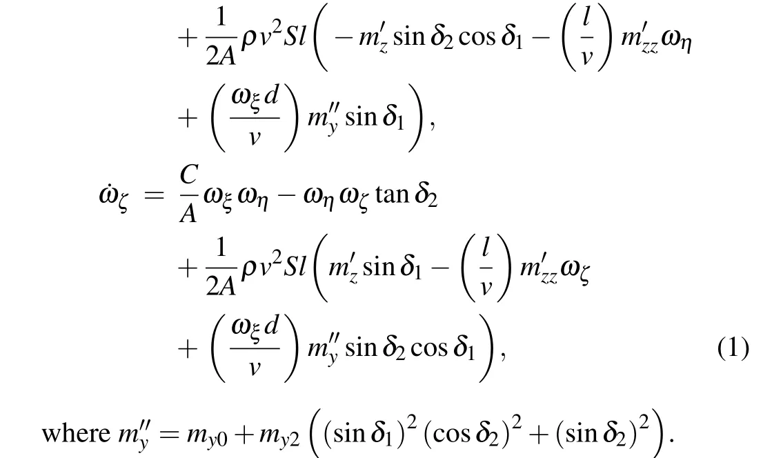
In order to generalize the data-driven method to the projectile systems， we simulate some sample path data based on the known model and identify the stochastic dynamical system from the data in this work. Formally， the angle motion equation of the projectile has the following form:[20]

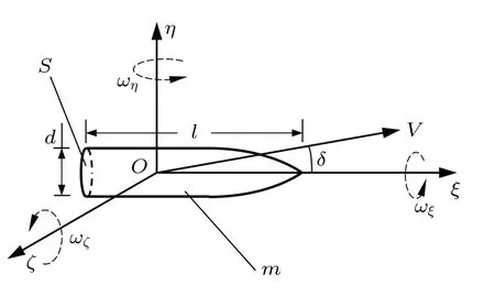
Fig.1. The model of the projectile system.

Here，ξ，ηandζdenote the three axes of the projectile coordinate system，Oξindicates the direction of the projectile axis，Oηpoints upwards and is perpendicular toOξ，andOζis perpendicular to the planeOξηpointing right. The state variablesωηandωζrepresent rotational angular velocity corresponding toηandζaxes，respectively. The other two variablesδ1andδ2indicate the vertical and horizontal components of the attack angleδ， which is the angle between the projectile axis and its velocity. The model of the projectile system with the axes and parameters is visualized in Fig.1.The structure and aerodynamic parameters in the equation are listed in Tables 1 and 2，respectively.

Table 1. Structure parameters.

Table 2. Aerodynamic parameters.

The variablevdenotes the velocity of the projectile during its flight in air， which can be easily influenced in general. In consideration of the random disturbances of air， the speed is assumed asv= ¯v+ξt，where ¯v=1012.3 m/s and the scalar stochastic processξtis a white Gaussian noise satisfying E[ξt]=0 and E[ξtξs]=2κδ(t-s). The noise intensity is chosen asκ=50 in the following computation.

Note that there exist some nonlinear terms about noise in Eq. (1). After the expansion of these nonlinear terms and neglecting of the higher order terms， we reduce it as the following standard Itˆo stochastic differential equation:

where the random vectorXt=[δ1，δ2，ωη，ωζ]T，the drift coefficient

and the diffusion coefficienta=σσTwith the functionσ，

3. Theory and method

According to the Fokker–Planck equation corresponding to stochastic differential equation (2)， the drift and diffusion coefficients dominate the probabilistic structure of the solution processXt.[21]Therefore， the discovery of the stochastic governing laws from sample path data completely depends on the identification of the drift and diffusion terms.

The Kramers–Moyal formulas can be used to extract the underlying stochastic dynamical systems from data，which express the drift and diffusion coefficients in terms of the sample paths of the solution process.[6，22]For our systems，these equations can be formulated as

wherebi(x)denotesi-th component of the drift vectorb(x)in Eq. (3)， andaij(x) indicatesij-th component of the diffusion matrixa(x). Then the driftb(x)and diffusiona(x)can be estimated by approximately computing the limit expressions on the right-hand side in terms of sample path data ofXt.

Assume that there exists a pair of data sets for the stochastic processXtcontainingMelements，respectively，

where everyyiis the image point ofxiafter a small evolution timehfori=1，2，...，M. In other words，Eq.(2)is integrated by numerical integral methods such as the Runge–Kutta method from initial pointxito getyiin timeh. Note that the superscript in Eq. (5) denotes different component of vector or matrix and the subscript in Eq.(6)indicates different data.It is also necessary to choose a dictionary of basis functionsΨ(x)=[ψ1(x)，ψ2(x)，...，ψK(x)]to approximate the drift and diffusion terms. The results will be better if we seek as rich type of the basis functions as possible， while the amount of work is immense and polynomial basis functions are sufficiently accurate for most cases. Thus we select polynomial functions as the dictionary in this research.

Assume that the system has ergodic property and every component of the drift coefficient is estimated asbi(x)=∑Kk=1cikψk(x)，i=1，2，3，4. Moreover， the limit expressions on the left-hand side of Kramers–Moyal formulas can be approximated by finite differences. Above all，we can derive the following group of linear equations via Eqs.(5)and(6):

The solution to Eq. (8) is generally very dense， which contains many non-dominant terms close to zero. For the sake of seeking the least coefficients without loss of reliability and avoiding overfitting，the sparse solution should be enforced by minimizing

whereρindicates a positive Lagrange multiplier to control the degree of sparsity.

We can use the iterating thresholding algorithm to realize the sparse learning method(9).[1，6，7]First， we can choose an appropriate pre-defined threshold parameterλas a sparsification knob. The magnitude ofλis usually chosen as about 0.1%–10%of the largest coefficient ofci. After Eq.(8)being performed to obtain a non-sparse solution， we set the coefficients smaller thanλas zero and delete the corresponding basis functions. Then the regression problem is carried out on the remaining coefficients. The procedure is iterated until no coefficients are found smaller thanλ.

Table 3. The algorithm for identifying the drift and diffusion terms from sample path data.

4. Results

In the above section，we described the data-driven method to extract the stochastic dynamical systems from sample path data based on the Kramers–Moyal formulas.We now show the effectiveness of this technique applied on the projectile system introduced in Section 2.

First， we chooseM=104initial points to construct the data setX， which are uniformly and randomly distributed in the region[-1，1]×[-1，1]×[-1，1]×[-1，1]. Given the time steph=0.0001， the image data setYis integrated via Euler scheme of the stochastic system(2). The dictionaryΨof basis functions is selected as the polynomial functions up to order 3，which contains 35 terms since the system is four-dimensional.Based on these preliminaries， we can compute the matrixAand vectorsBi，Bi jin Eqs.(7)and(10).

Via the least square method and sparse learning， all the components of the drift and diffusion coefficients are evaluated as the linear combination of the polynomial basis functions. Since the system is four-dimensional， it is impossible to show these functions intuitively in the figures. Thus we portray them as two-dimensional surfaces by fixing two state variables.

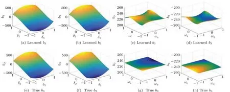
The learned and true functions of four components of the drift coefficient are shown in Figs.2–5，respectively. In every figure， the top panels denote the learned results and the bottom panels correspond to the true functions.The four columns of the figures indicate the cases with(i)ωη=0.5，ωζ=0.5;(ii)ωη=-0.5，ωζ=-0.5; (iii)δ1= 0.5，δ2= 0.5; (iv)δ1=-0.5，δ2=-0.5， respectively. It is seen that the estimation results agree well with the true functions of the drift terms. The third and fourth components have a small error but still within an acceptable range. This error stems from the fact that the magnitude of the two components is much larger than the first two. A coordinate transformation can lead to more accurate results.

As mentioned above， there are 10 elements of the diffusion matrix that need to be identified from data due to the symmetry. For the sake of simplification，we just present the diagonal elementsa11，a22，a33anda44for the case ofωη=0.5，ωζ=-0.5 in Fig. 6. The results show that the accuracy of the approximation of the diffusion term is not as good as the one for the drift coefficient， while it can still capture the dynamical structures. It seems that the errors fora11anda22are relatively larger. This is because the magnitude of them is too small to be sufficiently accurate. Above all，the identification of the stochastic dynamical system is consistent enough with the real model.

Fig.2. Comparison between learned and true function of the first component of the drift coefficient: (a)and(e)ωη =0.5，ωζ =0.5;(b)and(f)ωη =-0.5，ωζ =-0.5;(c)and(g)δ1=0.5，δ2=0.5;(d)and(h)δ1=-0.5，δ2=-0.5.

Fig.3. Comparison between learned and true function of the second component of the drift coefficient: (a)and(e)ωη =0.5，ωζ =0.5;(b)and(f)ωη =-0.5，ωζ =-0.5;(c)and(g)δ1=0.5，δ2=0.5;(d)and(h)δ1=-0.5，δ2=-0.5.

Fig.4. Comparison between learned and true function of the third component of the drift coefficient: (a)and(e)ωη =0.5，ωζ =0.5;(b)and(f)ωη =-0.5，ωζ =-0.5;(c)and(g)δ1=0.5，δ2=0.5;(d)and(h)δ1=-0.5，δ2=-0.5.

Fig.5. Comparison between learned and true function of the fourth component of the drift coefficient: (a)and(e)ωη =0.5，ωζ =0.5;(b)and(f)ωη =-0.5，ωζ =-0.5;(c)and(g)δ1=0.5，δ2=0.5;(d)and(h)δ1=-0.5，δ2=-0.5.

Fig.6. Comparison between learned and true function of the diagonal elements a11，a22，a33 and a44 of the diffusion matrix for ωη =0.5，ωζ =-0.5.

5. Conclusion

In summary， we have employed a data-driven method based on the Kramers–Moyal formulas to extract the stochastic model for the four-dimensional projectile systems from simulated sample path data. Specifically，the projectile system is assumed as an Itˆo stochastic differential equation. Then the least square method and sparse learning are applied to compute the drift coefficient and diffusion matrix， which are sufficiently accurate to the true functions. The effective approximation of the learned model to the real one implies that the data-driven method can be well applied to the projectile systems. Therefore， given the measurable time-series data， we can establish the governing equations for the projectile in the engineering field. This fact demonstrates that it has many applications in practical problems. For example， the learned model of the projectile can be used to analyze its dynamical responses so that we can improve the performances of the projectile by adjusting its shape and structure.

Acknowledgement

This research was supported by the Six Talent Peaks Project in Jiangsu Province，China(Grant No.JXQC-002).

Data availability statement

The data that support the findings of this study are openly available in GitHub.