Statistical prediction of waterflooding performance by K-means clustering and empirical modeling

Qin-Zhuo Lio ,Ling Xu ,Gng Li ,Xu Liu ,Shu-Yu Sun ,Shirish Ptil

a Department of Petroleum Engineering,King Fahd University of Petroleum and Minerals,Dhahran,Saudi Arabia

b Department of Petroleum Engineering,China University of Petroleum-Beijing,Beijing,102240,China

c Faculty of Engineering,China University of Geosciences,Wuhan,430074,Hubei,China

d Center for Integrative Petroleum Research,King Fahd University of Petroleum and Minerals,Dhahran,Saudi Arabia

e Department of Petroleum Engineering,King Abdullah University of Science and Technology,Thuwal,Saudi Arabia

Keywords:

ABSTRACT

1.Introduction

Reservoir simulation allows an engineer to evaluate various complex scenarios and predict the future reservoir performance(Aziz,1979;Wang et al.,2017;Lie,2019;Yavari et al.,2021;Rao et al.,2021).Obtaining direct measurements or hard data for the whole field is too expensive,even if possible.The geostatisticallybased approaches are usually used to generate multiple realizations of hydrodynamic parameters(Deutsch,2002).In the past several decades,statistical prediction methods for fluid flow and transport in porous media have been developed intensively and widely used in water resources engineering and oil production industry(Zhang,2001;Caers,2005;Lee et al.,2019;Xue et al.,2021).

In the numerical approaches,the widely used Monte Carlo(MC)method involves solving the forward model multiple times on random samples.Albeit robust and straightforward,it often requires an extremely large number of realizations to generate statistically accurate results and hence may become prohibitive,especially for large-scale models(Ballio and Guadagnini,2004).

Another alternative is the stochastic or probabilistic collocation method,which constructs polynomial approximation based on the model responses on selected collocation points(Li and Zhang,2007;Lin and Tartakovsky,2009;Xiu,2010;Liao and Zhang,2013).Specifically,the input random field is decomposed using the Karhunen-Loeve expansion/principle component analysis(Zhang and Lu,2004),and the output random field is approximated via the Lagrange interpolation or orthogonal basis function,whose coefficients are solved by pseudo-spectral projection or matrix inversion(Le Maître and Knio,2010).It is found to be quite promising for low-to moderate-dimensional models using Smolyak sparse grids(Xiu and Hesthaven,2005;Liao et al.,2017b).

However,for some large-scale reservoir models,we can only afford to run several(usually of order O(1))realizations.In contrast,the number of required realizations are usually of order O(10),when the correlation length is relatively large compared to the domain size(Liao et al.,2017a).It can be even worse if the correlation length is much smaller than the domain size,where the eigenvalue will decay at a very slow rate and hence the truncation error will be very large if some of the terms are neglected.Thus,a large number of orthogonal bases have to be retained with an exponential growth of computational cost,which is the wellknown“curse of dimensionality”.

In this study,we propose to use the single-phase flow solutions to approximate the two-phase flow solutions,which will provide a significant speed-up without losing much accuracy.Specifically,instead of carrying out time-intensive two-phase flow simulations for a large number of realizations,we first perform single-phase flow simulations on all these realizations,then use K-means clustering to choose one representative in each group,and perform two-phase flow simulations on the representatives only.These two-phase flow simulations(on the representatives)and singlephase flow simulations(on all these realizations)allow us to get the empirical models,which are used to predict the two-phase solutions in all realizations.

The idea in this study is similar to the decline curve analysis(DCA),which is a reservoir engineering empirical technique that extrapolates trends in the production data from oil and gas wells(Arps,1945;Fetkovich,1980;Doublet et al.,1994;Fetkovich et al.,1996;Agarwal et al.,1998).The purpose of a DCA is to generate a forecast of future production rates and to determine the expected ultimate recoverable reserves.Our proposed method also uses the empirical models for prediction,but estimates the production data in multiple realizations.That is,we approximate the dependent variables in stochastic/parametric domain instead of the temporal domain.

This paper is organized as follows:In Section 2,we introduce the governing equations.In Section 3,we present the proposed method using K-means clustering and empirical modeling.In Section 4,we validate the method by comparing it to the MC simulation in twodimensional(2D)and three-dimensional(3D)examples under different well control conditions.Section 5 discusses several issues including different choices of empirical models,effect of the number of clusters,etc.Finally,Section 6 draws the main conclusions.

2.Governing equations

The steady-state,single-phase flow satisfies the following continuity equation(Bear,1972)

whereρis density,u is velocity,and q is the source/sink term.Darcy's law for single-phase flow is

where k is the absolute permeability,μis viscosity,p is pressure,g is the gravitational acceleration,z is depth.

The waterflooding model can be expressed by the following equation(Bear,1972)whereφis the porosity;and each phase has its own densityρα,saturation Sα,phase velocities uα,and source term qα.Darcy's law for multiphase flow is

where krα,μα,and Pαare the relative permeability,viscosity,and pressure for phaseα,respectively.Eqs.(3)and(4)are usually coupled with

where Pcis the capillary pressure;which is a function of Sw.

In geostatistics,the absolute permeability is considered as a random field.Specifically,the ln-permeability is usually treated as a stationary Gaussian random field with a mean and an exponential covariance of(Dagan,1989)

3.Methodology

3.1.K-means clustering

K-means clustering is an unsupervised machine learning method for the classification of unlabeled data into groups and determining cluster centers.One chooses the desired number of clusters,and the K-means procedure iteratively moves the centers to minimize the total within-cluster variance.Specifically,the criterion is minimized by assigning the observations to the K clusters in such a way that within each cluster the average dissimilarity of the observations from the cluster mean,as defined by the points in that cluster,is minimized(Hastie et al.,2009).

Consider a set of p-dimensional vector{xi}={xi1,xi2,…,xip},and the dissimilarity measure follows the squared Euclidean distance

The objective is to find

where Nkis the number of points in cluster k,is the center of cluster k,C(i)=k indicates xibelongs to cluster k.Given an initial set of centers,the K-means algorithm alternates the two steps:(1)for each center we identify the subset of training points(its cluster)that is closer to it than any other center;(2)the means of each feature for the data points in each cluster are computed,and this mean vector becomes the new center for that cluster.These two steps are iterated until convergence.Typically,the initial centers are randomly chosen observations from the training data.Details of the K-means procedure,as well as generalizations allowing for different variable types and more general distance measures,are given in Hastie et al.(2009).

3.2.Empirical modeling

The DCA is a graphical procedure used for analyzing declining production rates and forecasting future performance of oil and gas wells.Fitting a line through the performance history and assuming this same trend will continue in future forms the basis of the DCA concept.

Our empirical modeling shares a similar idea and uses the single-phase flow rate q as the independent variable rather than time.That is,we approximate the dependent variables in stochastic/parametric domain instead of the temporal domain.The idea is based on the following thinking:the oil production rate qoin twophase flow can be considered as a function of permeability and time as qo=qo(k,t),assuming that the permeability k is a constant(e.g.,in homogeneous media)for simplicity.The traditional DCA treats qoas a function of time as qo=qo(t)for a given realization of the permeability field k.Similarly here,we may treat qoas a function of permeability as qo=qo(k)at a certain time t.In addition,we have q=q(k)from the single-phase flow simulation.Now we can relate qoand q(via permeability k)as qo=qo(q)at a certain time t.Note that the Darcy's law states that the relationship between the permeability and flow rate is a linear relation,in both single-phase and multiphase flows.For example,if k is doubled,both q and qowill be doubled.That is,qowill be linear/proportional to q,when k varies.Here we just use the oil production rate as an example,while the water production rate or injection rate can be considered as well.

The above analysis is based on ideal conditions(e.g.,homogeneous media,linear relative permeability,neglecting capillarity and gravity).Although these conditions may not be satisfied in complicated examples,the linear relation between the rate of single-phase flow and the rate of multiphase flow still plays a dominant role.We will show in the case studies that this idea actually works well in heterogeneous media with quadratic relative permeability,considering capillarity and gravity.

In waterflooding applications,we are usually interested in the water injection rate,oil and water production rates,as well as the well bottom-hole pressure(BHP).Note that the total production rate,which is the sum of oil rate and water rate(i.e.,qt=qo+qw),has a relatively linear relation with the single-phase rate q.Therefore,we propose to approximate qtand the fractional flow fw,and then use them to compute qoand qw.

To account for the nonlinear effect besides the dominant linear relation(since the ideal conditions are not satisfied in general),a quadratic function can be used for qtas

where a,b and c are constant coefficients.Physically,for zero capillarity,if q is 0,indicating vanishing connectivity(e.g.,a barrier)between the injector and the producer,and thus qtshould be 0 as well.Thus,the coefficient c should be 0.Note that if the injection well is controlled by a fixed injection rate,then the well BHP can be approximated by a quadratic function.To determine the above coefficients,we may use least-squares regression to solve this overdetermined problem,considering that it is a system of linear equations.

As for the fractional flow fw,it can also be viewed as a function of permeability and time as fw=fw(k,t).In a deterministic model where the permeability k is fixed,fw=fw(t)is 0 before water breakthrough and monotonically increases with time afterwards.Alternatively,we may view fwas a function of k,i.e.,fw=fw(k),at any given time.Then,considering the relation of q and k via singlephase flow,fwcan be expressed as fw=fw(q)as well.Specifically,fwremains 0 for a small q,increases as k grows after water breakthrough,and finally approaches 1 as q approaches infinity.We thus propose to use the exponential function with truncation as

where a and b are constant coefficients that determine the shift and curvature,respectively.Note that Eq.(10)is based on the assumption that the water/oil mobility ratio is close to unity,under which the single-phase flow rate becomes a good approximation of the total rate in the two-phase flow.Since Eq.(10)is a nonlinear equation,we may use the function“fminsearch”in MATLAB,which finds the minimum of unconstrained multivariable function using derivative-free method,to determine the coefficients a and b.

We remark that the analytical solution of fwexists for incompressible two-phase flow in homogeneous media with negligible capillary pressure effects and gravitational forces,which is the well-known Buckley-Leverett theory.In particular,if the relative permeability is concave upward(which is often the case),the saturation profile will consist of a shock wave followed by a rarefaction wave.Based on this,it seems that the empirical function for fwshould include a discontinuous section to mimic the shock front.However,in reality,the saturation profile is usually smoothened and continuous due to physical dispersion(e.g.,caused by capillarity)and/or numerical dispersion(Lei et al.,2020).Therefore,the continuous formula as in Eq.(10)is suggested.

Actually,we tested some other empirical models(e.g.,cubic function for qt,and reciprocal function for fw),and found that Eqs.(9)and(10)are the best formulas in general.This is consistent with the observations in DCA,where the exponential function is probably the most widely used decline curve model.More detailed discussions for this issue are included in the case studies.

3.3.Proposed method

This study proposes a new approach for predicting the statistics of waterflooding performance.The key idea is to combine a small number of two-phase flow simulations(which is time consuming)and a large number of single-phase flow simulations(which is much faster).Specifically,we first randomly generate a large number of realizations,perform single-phase flow simulations and obtain the production rates.And we use the K-means clustering technique to divide the realizations into a few groups,and choose one representative realization in each group.We then perform twophase flow simulations on these representative realizations and obtain the corresponding model responses including total production rate and fractional flow.After that,we fit the empirical models using responses data,which can be used to predict the model responses in other realizations.

The complete algorithm is presented as below:

Algorithm 1.K-means clustering and empirical modeling

1 Randomly generate a large number of realizations(Eq.(6)).

2 Perform single-phase flow simulations on all realizations(Eq.(1)and(2)).

3 Use K-means clustering and choose one representative in each group(Eq.(8)).

4 Perform two-phase flow simulations on the representatives(Eqs.(3)-(5)).

5 Fit the empirical models for pressure/total rate and fractional flow(Eq.(9)and(10)).

6 Use the empirical models and single-phase solutions to predict the two-phase solutions.

In this work,we use the MATLAB Reservoir Simulation Toolbox(MRST)(Lie,2019)for the single-phase flow simulation and the Schlumberger ECLIPSE simulator for the two-phase simulation.We use the MATLAB build-in functions“kmeans”for K-means clustering and“fminsearch”for curve fitting.

4.Case studies

4.1.Base case

In this section,the idea and procedure of the proposed method are illustrated by a 2D example in a quarter five-spot pattern.The 2D space of 600×600×20 ft3is divided into 30×30×1 gridblocks,with each 20×20×20 ft3.No-flow boundary condition is applied to all bounds.The porosity is assumed constant at 0.15.The absolute ln-permeability(in mD)is a stationary Gaussian random field with a mean of 3.0,and a variance of 1.0.The spatial correlation follows an exponential covariance function with the correlation lengths of 60 ft and 120 ft in the x-and y-directions,respectively.The Coreytype relative permeabilities are represented by quadratic functions as krw=and kro=(1-Se)2,where,Seis the effective saturation,Se=(Sw-Swi)/(1-Sor-Swi),where Swiis the irreducible water saturation and Soris the residual oil saturation.The following values are used in this study:Swi=0∙2,Sor=0∙3.The capillary effect is neglected in this case(Case 1).There is one injector and one producer,controlled by fixed BHPs at 5000 psia and 3000 psia,respectively.The locations of the wells are shown in Fig.1,which also illustrates one realization of the ln-permeability field randomly generated using geostatistics.

In the traditional MC method,we randomly generate 1000 realizations of the ln-permeability field and perform waterflooding simulations for each of them up to 500 days.Thus,we have 1000 samples of model responses(e.g.,water injection rate,oil production rate and water production rate).

In our proposed method,we first run the single-phase simulation for the 1000 realizations and obtain the injection and production rates.These two rates are then clustered using the K-means clustering as shown in Fig.2.In this synthetic example,the injection rate and production rate(in single-phase flow)are exactly the same,owing to mass balance.Therefore,the data points in Fig.2 fall on a straight line.We set a number of clusters(10 in this study),and in each cluster,one point that is closest to the cluster center is selected to represent the cluster center.Hence,these 10 points(i.e.,10 realizations)serve as representatives in the following analysis.

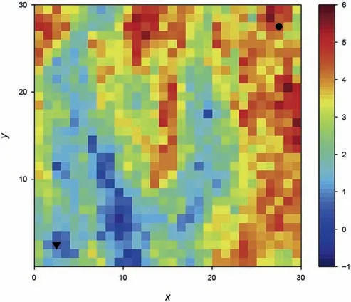
Fig.1.One realization of ln-permeability(in mD)field in the 2D test.The triangle indicates injector,and the circle indicates producer.

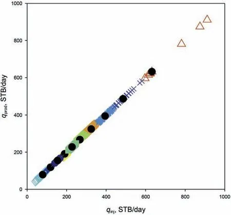
Fig.2.Ten clusters from K-means clustering in the 2D test.The data points in ten clusters are plotted by ten different markers and colors.The solid black circles indicate the closest points to each cluster center.

We then perform waterflooding simulation for these 10 realizations and thus have 10 samples of model responses.Fig.3a shows the total production rate qtat time t=200 days.The green dots are from 1000 MC simulations.The red circles are the 10 points selected from clustering.The blue curve is the quadratic function from curve fitting using the 10 points.Note that the total production rate qtshould be zero if the single-phase production rate q is zero,based on physics,and thus the intercept in the quadratic function is set to be zero.In addition,qtis different from q(even for the same field as in this test)mainly because of the relative permeability and heterogeneity.Specifically,as the sum of relative permeabilities is no greater than one,qtwould be smaller than q in general.Fig.3b shows the fractional flow fwat time t=200 days.The 10 points are fitted using an exponential function.We can see that the fitted curves match the exact responses quite well.Once the fitted curves are determined(i.e.,the coefficients are solved from regression),we may use them as proxy models to generate 1000 samples of the responses conveniently.

For each time step,the above process is implemented,until we obtain all required data samples.Now we have the model response samples in all time steps,and can easily estimate their statistics.It is customary in the petroleum industry to describe the uncertainty in terms of P10,P50 and P90,where the“P”stands for percentile.For example,P10 means that 10%of the calculated estimates will be no greater than the P10 estimate.Usually,P10 indicates the low estimate,P50(i.e.,median)indicates the best estimate,and P90 indicates the high estimate.Fig.4 shows these results for the total production rate and the fractional flow.The black solid lines are from 1000 MC(two-phase flow)simulations and considered as the exact results.The red dash-dotted lines are from 10 MC(two-phase flow)simulations for comparison.The blue dashed lines are from our proposed method,i.e.,using 10(two-phase flow)simulations and 1000(single-phase flow)simulations.We can see that the results from our proposed method generally agrees well with the exact results,and is much better than those from the MC method with 10 simulations.

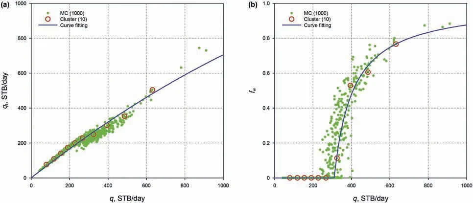
Fig.3.Empirical models and curve fitting:(a)total production rate in waterflooding as a function of single-phase production rate,fitted by a quadratic function;and(b)fractional flow in waterflooding as a function of single-phase production rate,fitted by an exponential function with truncation.

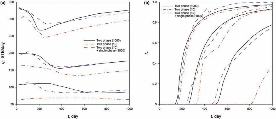
Fig.4.Exact and estimated P10,P50 and P90:(a)total production rate;and(b)fractional flow.

Usually we are more interested in the oil and water rates than the total rate and fractional flow,since the formers have better practical meanings in real applications.Actually,the latter ones can be computed easily from the former ones as qo=qt×fwand qw=qt×(1-fw).Their results are depicted in Fig.5.We can see that the MC method with 10 simulations clearly underestimates the variabilities,whereas the proposed method performs reasonably well.

We remark that the qwline of P10 in Fig.5b is close to 0,till the end of simulation.It is indeed true that the qwvalues remain unchanged in around 100 realizations.While in Fig.5a,the qoline of P10 still decreases,mainly due to the relative permeability.Since the quadratic functions krw=S2eand kro=(1-Se)2are used in this study,krw+kro≤1.Considering that initially the oil saturation reaches maximum and then gradually decreases,the total flow rate qtwill decrease as well.Therefore,even qwremains zero,qowill still generally decrease with time.

To further analyze the distribution of oil and water rates,we compare the cumulative density functions(CDFs).Fig.6 reveals the results at time t=200 days.The red lines behave in a zig-zag manner since there are only 10 samples in the MC method.In comparison,the blue lines almost overlap the black lines,indicating a high accuracy of the proposed method.

4.2.Effect of capillarity

To analyze the effect of capillarity,we test another case(Case 2).Consider the capillary pressure as Pc=1/Se-1/(1-Se)shown in Fig.7.Other conditions are the same with those in Case 1 above.We even use the same ensemble of 1000 realizations.In general,the results are very close to those in Case 1.For example,the P10,P50 and P90 of the total production rate and fractional flow are depicted in Fig.8,which is similar to Fig.4.To quantitatively compare the differences in Case 1 and Case 2,we compute the errors of the mean and standard deviation in a relative error sense as

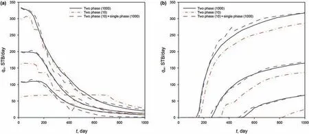
Fig.5.Exact and estimated P10,P50 and P90:(a)oil production rate;and(b)water production rate.

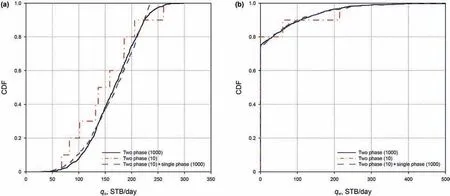
Fig.6.Exact and estimated cumulative density function(CDF):(a)oil production rate;and(b)water production rate.

where the summation w.r.t.t is to account for all time steps.The results for the proposed method are illustrated in Table 1,considering the MC method with 1000 realizations as the exact reference.It is seen that the proposed method is at the same level of accuracy in Case 2(with capillarity)as in Case 1(without capillarity).

4.3.Effects of heterogeneity,variability and mobility ratio

We then compare the results from the proposed method and the MC method under various conditions,including heterogeneity,variability,and mobility ratio(Table 1).We consider Case 1 as the base case,and change the parameters one at a time,to investigate 6 difference case(Cases 3-8).Specifically,the correlation lengths are changed in Cases 3 and 4;the variance of log-permeability is changed in Cases 5 and 6;and the mobility ratio is changed in Cases 7 and 8.

Table1 Relative error of the mean and standard deviation of the total production rate qt and fractional flow fw in Cases 1-8.

The errors of the mean and standard deviation of the total production rate qtand fractional flow fware summarized.It can be seen that the proposed method is mostly affected by the mobility ratio,but not affected much by the heterogeneity or variability.This can be explained as the proposed method assumes that the mainly features of the two-phase flow can be captured by the single-phase flow,and thus works better when the mobility ratio is close to unity.In most reservoir situations,water viscosity is lower than oil viscosity,making the viscosity ratio unfavorable for water to displace oil efficiently.However,the relative permeability of water at residual oil saturation could be lower by a factor of two to eight than that of oil at connate-water saturation.Hence,for many reservoirs,the mobility ratio is close to unity if the oil viscosity is greater than the water viscosity at reservoir conditions by a factor of five or so.In general,we can see that the proposed method is more accurate than the traditional MC method with the same amount of computational cost.

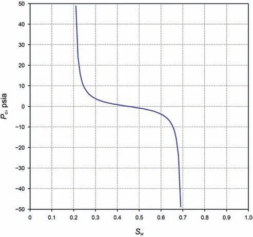
Fig.7.Capillary pressure as a function of water saturation.

4.4.Channelized system

In this section,the proposed method is tested using a more challenging/realistic geo-statistical model:a channelized system.We use the open source Stanford Geostatistical Modeling Software(SGeMS)for the application of multi-point geostatistics.Fig.9a displays the widely-used training image,which is defined on a 250×250 grids and characterizes the geological features(spatial correlation structure)and thus the multipoint statistics.A total of 1000 conditional SGeMS realizations are generated using the single normal equation simulation(SNESIM)algorithm(Strebelle,2002).Fig.9b shows four realizations and each contains 50×50 grids.The red and blue colors correspond to sand(k=100 mD)and mud(k=1 mD)facies,respectively.There are two injection wells and three production wells,whose locations are indicated in Fig.9b.All realizations are not conditioned to hard data at these well locations,thus high uncertainty in the production data is expected.The other conditions are the same as in the base case in Section 4.1.

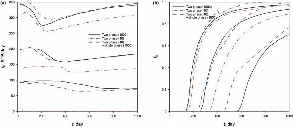
Fig.8.Exact and estimated P10,P50 and P90 in Case 2 with capillarity:(a)total production rate;and(b)fractional flow.

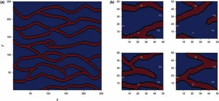
Fig.9.Illustration of channelized reservoirs:(a)training image;and(b)4 randomly generated realizations.

Fig.10.Exact and estimated P10,P50 and P90 in the channelized field case:(a)oil production rate at well P1;and(b)water production rate at well P1.

Fig.10 displays the P10,P50 and P90 responses for oil and water production rates at well P1 obtained from the proposed model and MC method.Significant differences between the reference(in black)and the MC method with 10 simulations(in red)are evident for this challenging case,especially for the P90 estimations.These discrepancies are mainly because the channel connectivity in all 1000 realizations cannot be captured by only 10 simulations,and the fact that the wells in these simulations are under BHP control.It appears that the P10 and P50 lines are close to zero,since their values are too small compared to P90 values,which is also validated by the CDF curves as shown in Fig.11.The proposed method,however,is found to be consistent with the reference in both figures.

4.5.Three-dimensional test

In this section,the proposed method will be tested in a more complicated 3D example with five wells.Consider a space of 820×820×20 ft3is divided into 41×41×10 gridblocks,with each 20×20×2 ft3.The porosity is assumed constant at 0.2.No-flow boundary condition is applied to all bounds.The absolute lnpermeability(in mD)is a stationary Gaussian random field with a mean of 3.0,and a variance of 1.0.The spatial correlation follows an exponential covariance function with the correlation lengths of 100,50,and 4 ft in the x-,y-and z-directions,respectively.The same relative permeabilities as in the 2D example are used here,and the capillarity is neglected.There is one injector in the center controlled by an injection rate of 1000 STB/day,and four producers all controlled by BHPs of 2000 psia.All wells penetrate 10 layers.Fig.12 illustrates one realization of the ln-permeability field randomly generated using geostatistics,with the well locations.

In the MC method,we still generate 1000 realizations of the lnpermeability field randomly,and perform waterflooding simulations for each of them up to 600 days.We hence have 1000 samples of model responses,including injection well BHP and production rates.

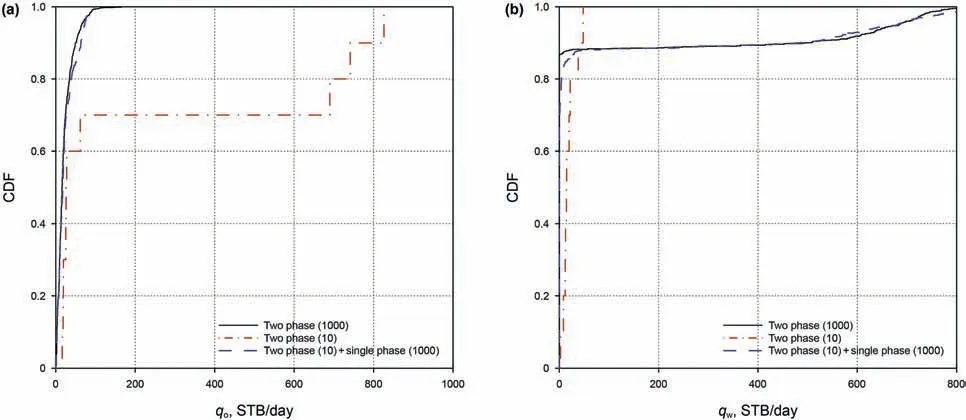
Fig.11.Exact and estimated cumulative density function(CDF)in the channelized field case:(a)oil production rate at well P1;and(b)water production rate at well P1.

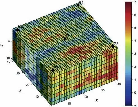
Fig.12.One realization of ln-permeability(in mD)field in the 3D test.The triangle indicates injector,and the circles indicate four producers.

In our proposed method,we also run the single-phase simulation for the 1000 realizations and obtain the injection well BHP and the rates at four production wells.These five responses are then clustered using the K-means clustering as shown in Fig.13.In this example,the injection rate is fixed,and thus the summation of the four production rates is fixed.Therefore,there are 5-1=4 independent variables(including injection well BHP).Although the clustering result cannot be shown in a 4D space,it can be partially illustrated in a 2D space(with two independent variables,e.g.,production rates at P1 and P2).Note that the variables have to be normalized(by their individual standard deviations)to make them equally weighted before clustering.We still use 10 clusters,and select 10 points/realizations as representatives in the following analysis.

Fig.14 shows the empirical models and curve fitting for well P1 at time t=200 days.While the total production rate is reproduced accurately by a quadratic function,there are some mismatches in the fractional flow,especially when the fractional flow is close to zero.This is because the data points are more clustered(due to multiple production wells)than those in the 2D example.After using empirical functions to fit the data,we may generate a large number of samples readily,from which the model output statistics can be calculated.Fig.15 presents the P10,P50 and P90 for the oil and water production rates.The injected pore volume is larger in this 3D example than in the 2D example,and hence the oil rate is reduced to a lower level.The variance of the production rates is smaller than those in the 2D example,mainly because the injection well control condition is changed from constant BHP to constant injection rate.The other three production wells perform similarly and thus will not be shown repeatedly.

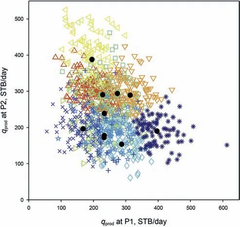
Fig.13.Ten clusters from K-means clustering in the 3D test.The data points in ten clusters are plotted by ten different markers and colors.The solid black circles indicate the closest points to each cluster center.

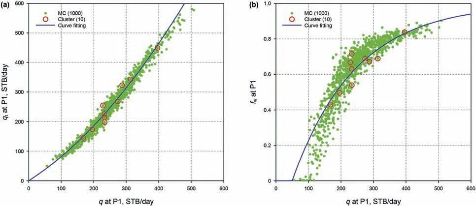
Fig.14.Empirical models and curve fitting at well P1:(a)total production rate as a function of single-phase production rate,fitted by a quadratic function;and(b)fractional flow as a function of single-phase production rate,fitted by an exponential function with truncation.

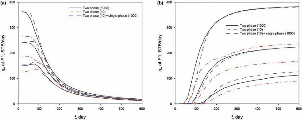
Fig.15.Exact and estimated P10,P50 and P90 at well P1:(a)oil production rate;and(b)water production rate.

Different choices of empirical models may affect the accuracy of prediction.For the estimation of the multiphase flow rate or BHP using the single-phase flow rate,the dominant feature is a linear relation,as shown in Figs.3a,14a and 16.Therefore,a quadratic function performs very well in approximating the model responses(at both injection and production wells).However,for the fractional flow or water cut,its behavior is more complicated and highly nonlinear,as shown in Figs.3b and 14b.Similar to the DCA,in which there are three types of declines(i.e.,exponential,hyperbolic and harmonic),we have three choices here as well.The main difference is that:the fractional flow for water is increasing here rather than decreasing as in the DCA.Specifically,both the exponential function(similar to the exponential decline)and the reciprocal function(similar to the harmonic decline)seem to work adequately,but the exponential function appears to be slightly better than the reciprocal function in general cases.The third choice(similar to the hyperbolic decline)is also tested,but is found to be inaccurate(detailed results are not shown due to limited space),mainly because it contains an additional unknown coefficient,considering the limited number of data points.That is,the result is more likely to be unstable when determining three unknowns by fitting ten data points,compared to two unknowns in the exponential or reciprocal function.

For the injection well,since the water injection rate is fixed,we compare the BHPs from three approaches.The relation between the single-phase BHP and two-phase BHP should be close to linear relation according to Darcy's law.The quadratic function is used as the empirical model and works very well,as shown in Fig.16.Fig.17 reveals the P10,P50 and P90,as well as the CDF of the injection well BHP(at t=200 days).A nice agreement between the exact values and the proposed results is observed in all these plots.In contrast,the MC method with 10 realizations generally underestimate the variability of the model outputs.This can be explained as when the number of samples is too small,it is difficult for the MC method to“hit”the sample that is far from the mean.

Lastly,we compare the CPU time(on the Intel Core i7-6700K CPU@4 GHz):the traditional MC method with 1000 realizations takes 203 min,whereas the proposed method takes 222 s,including 87 s for 10 two-phase flow simulations and 135 s for 1000 single-phase flow simulations,which is about 55 times faster than the MC method in the computational cost.We remark that it is indeed true that the 10 two-phase simulations took 87 s(8.7 s for each on average),while the 1000 simulations took 203 min(0.2 min=12 s for each on average).Although it appears that the CPU time for two-phase flow simulations is not stable,this is actually because the computational cost is related to the convergence rate,which is affected by the heterogeneity of the random field.In general,if the domain is more heterogeneous,it takes more time in simulation.Therefore,considering that these 10 simulations are so selected that present the cluster centers,their average CPU cost will be smaller than that from all 1000 random realizations,as can be seen from Fig.13(q can be viewed as a heterogeneity indicator).

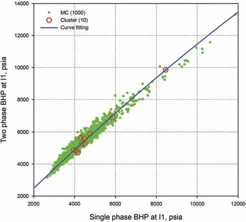
Fig.16.Empirical models and curve fitting at well I1:bottom-hole pressure(in twophase model)as a function of bottom-hole pressure(in single-phase model),fitted by a quadratic function.

4.6.SPE10 large-scale test

In order to test the proposed method in more complex geological models with higher simulation costs,we adopt the SPE10 benchmark project(Christie and Blunt,2001),which is widely employed for reservoir simulation.The fine-scale geological model is described on a regular Cartesian grid,with a domain size of 1200×2200×170 ft3.It has 60×220×85 cells,and each size is 20×10×2 ft3.The top 35 layers exhibit Gaussianity in logpermeability data,whereas the bottom 50 layers are channelized.In this study,we select the top 10 layers.Since the type of covariance function is not known,we performed variogram analysis,and found that the spherical covariance provides the best fit with the parameters as:σ2y=5∙0,ηx=600 ft,ηy=600 ft,andηz=10 ft.We set 2 injectors at constant BHP of 8000 psia and 13 producers at constant BHP of 4000 psia(as two nine-spot patterns),penetrating all 10 layers,as shown in Fig.18.This benchmark project is wellknown for its extremely large variance in the permeability field(about 6 orders of magnitude),as can be seen in Fig.18.Other information is as described in Christie and Blunt(2001).The simulation is performed up to 2000 days.

Fig.19 depicts the field oil and water production rates.We can see that the proposed method using 16 clusters/representatives match the reference with 800 simulations well,but the MC method with 16 simulations clearly deviate from the exact results.In this test,we used a 16-core Intel Xeon processor for parallelization,and each two-phase flow simulation takes about 10 min,while the single-phase flow simulation become negligible in computational time.Therefore,the proposed method using 16 clusters requires roughly 10 min.On the other hand,the exact results using 800 simulations require 10 h,even with parallelization,which is about 60 times slower than the proposed method.

We also test the effect of the number of clusters.If we use five clusters,the underdetermined problem(data points are not enough to determine the fitting parameters)will be likely to appear,although its performance is still better than the traditional MC method.If we use many clusters(e.g.,over a hundred),the proposed method will be more accurate but limited by the empirical models,and thus may lose advantage over the traditional MC method.We remark that the well control conditions should be fairly stable when using this method,otherwise,the empirical model may not be appropriate,which is the same as in the DCA.

We remark that the results from a small sample of MC simulations underestimates oil and water production rates in the above case studies.Actually,this underestimation is not always true,and overestimation is also possible as we have seen in some cases.However,underestimation is indeed more likely to appear than overestimation.This is because the production rate is essentially proportional to permeability,and permeability is log-normally distributed(right-skewed).Considering that the samples are randomly generated from a right-skewed distribution,the mean of these samples is likely to be lower than the exact mean value.

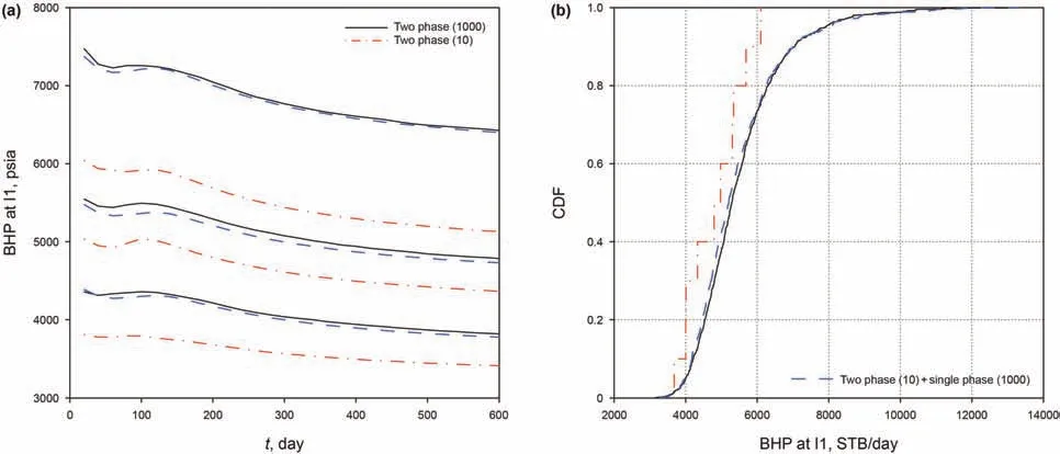
Fig.17.Exact and estimated values of bottom-hole pressure at well I1:(a)P10,P50 and P90;and(b)cumulative density function(CDF).

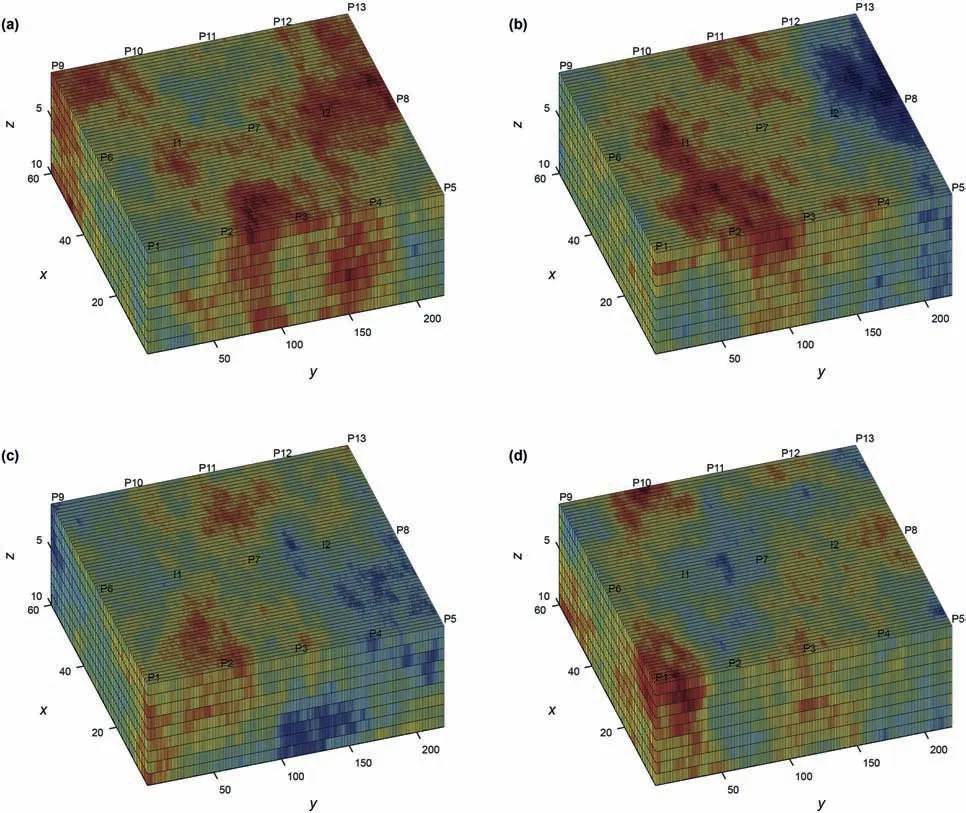
Fig.18.Illustration of 4 randomly generated realizations of permeability(in mD)field in the in the SPE10 case:(a)K realization 1;(b)K realization 2;(c)K realization 3;and(d)K realization 4.“I”indicates injector,and“P”indicates producer.

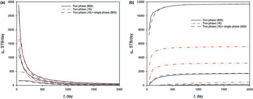
Fig.19.Exact and estimated values of field production rates:(a)oil rate;and(b)water rate.

5.Discussion

The proposed method is related to the concept of reduced-order modeling(Benner et al.,2015;Li et al.,2021),which involves simplifications of high-fidelity,complex models by capturing a system's dominant behavior and effects using minimal computational resources.In general,reduced-order modeling via surrogate models can be categorizes into two different classes:data-fit models and physics-based models.Data-fit models include response surface methods(e.g.,polynomial,radial basis function and kriging,etc.)that use interpolation or regression to fit a proxy model for the system output as a function of the input parameters.Physics-based models derive hierarchical surrogates from highfidelity models by,e.g.,simplifying physics assumptions(Wilson and Durlofsky,2013)and using coarser grids(Durlofsky,1991),aiming for reduced computational cost(and possibly lower accuracy).Our proposed method can be viewed as a reduced-physics modeling,where the single-phase flow solutions are utilized to approximate the multiphase flow solutions.As far as we know,this idea has not been proposed before.

For the single-phase flow simulation,we may use either water or oil,as long as the fluid is slightly compressible,since it is the relative value that matters instead of the absolute value,considering that the single-phase solution is just used for fitting/interpolation.Strictly speaking,using a transient state instead of a steady state in the single-phase flow simulation would provide better results,since the former is closer to the multi-phase flow(which is also transient)than the latter.However,the improvement is not significant in general cases.Considering that the computational cost is also increased if the transient state is used,we suggest using the steady state for single-phase flow simulations.

We are currently investigating possible extensions,e.g.,black-oil models,inverse problems(Neuman et al.,2012;Xue and Zhang,2014;Dai et al.,2016;Liao et al.,2019a),and other unsupervised learning approaches(Amir et al.,2020;Sun and Zhang,2020).This method can also be combined with the upscaling methods(Liao et al.,2019b,2020)for even higher efficiency.

6.Conclusions

A new approach,K-means clustering assisted empirical modeling,is presented for efficiently estimating waterflooding performance for multiple geological realizations.In this approach,the two-phase flow problems are numerically calculated for a small portion of realizations selected by the K-means clustering.For the majority of realizations,only the single-phase flow problems are solved.The empirical models are then used to relate the singlephase solutions and the two-phase solutions on these small portion of realizations.Finally,the two-phase solutions in other realizations can be predicted using the empirical models.

The proposed method is easy to understand and implement.It aims to achieve agreement at the ensemble level between the single-phase and two-phase flow simulation models,as can be seen from the P10,P50 and P90 results.Actually,it also performs well in the realization-by-realization agreement,indicated by the cumulative density function comparisons.The method is applied to both 2D and 3D synthetic models,and channelized reservoir and SPE10 benchmark test,with or without capillarity,considering different number of wells and control conditions,as well as the effect of heterogeneity,variance of log-permeability and mobility ratio.It is found that the proposed method is best for unit mobility ratio,and it consistently improves the Monte Carlo(MC)predictions with a few simulations and is able to capture the ensemble statistics of the MC results with a large number of realizations,while the computational cost is significantly reduced.

Acknowledgements

The authors in China would like to thank the funding supported by Beijing Natural Science Foundation(Grant No.3222037),the PetroChina Innovation Foundation(Grant No.2020D-5007-0203)and by the Science Foundation of China University of Petroleum,Beijing(Nos.2462021YXZZ010,2462018QZDX13,and 2462020YXZZ028).