THE GLOBAL EXISTENCE AND A DECAY ESTIMATE OF SOLUTIONS TO THE PHAN-THEIN-TANNER MODEL*

Ruiying WEI (位瑞英)

School of Mathematics and Statistics，Shaoguan University，Shaoguan 512005，China

E-mail:weiruiying521@163.com

Yin LI (李银)†

Faculty of Education，Shaoguan University，Shaoguan 512005，China

E-mail:liyin2009521@163.com

Zheng-an YAO (姚正安)

Department of Mathematics，Sun Yat-sen University，Guangzhou 510275，China

E-mail:mcsyao@mail.sysu.edu.cn

Abstract In this paper，we study the global existence and decay rates of strong solutions to the three dimensional compressible Phan-Thein-Tanner model.By a refined energy method，we prove the global existence under the assumption that the H3 norm of the initial data is small，but that the higher order derivatives can be large.If the initial data belong to homogeneous Sobolev spaces or homogeneous Besov spaces，we obtain the time decay rates of the solution and its higher order spatial derivatives.Moreover，we also obtain the usual Lp-L2(1≤p≤2) type of the decay rate without requiring that the Lp norm of initial data is small.

Key words Phan-Thein-Tanner model;global existence;time decay rates

1 Introduction

The theory of the Phan-Thein-Tanner model has recently gained quite some attention，and is derived from network theory for polymeric fluid.This type of fluid is described by the following set of equations:

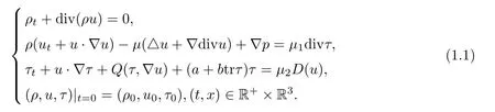
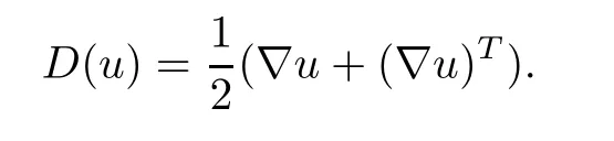
The unknownsρ，u，τ，pare the density，velocity，stress tensor and scalar pressure of the fluid，respectively.D(u) is the symmetric part of∇u;that is，

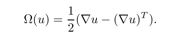
Q(τ，∇u) is a given bilinear form

where Ω(u) is the skew-symmetric part of∇u，namely，

μ＞0 is the viscosity coefficient andμ1is the elastic coefficient.aandμ2are associated with the Debroah number(which indicates the relation between the characteristic flow time and elastic time[2]).λ∈[-1，1]is a physical parameter;we call the system a co-rotational case whenλ=0.b≥0 is a constant related to the rate of creation or destruction for the polymeric network junctions.

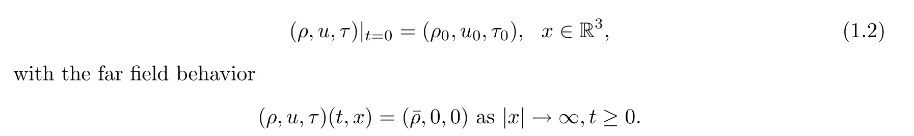
To complete system (1.1)，the initial data are given by

Let us review some previous works about model (1.1) and related models.If we ignore the stress tensor，(1.1) reduces to the compressible Navier-Stokes (NS) equations.The convergence rates of solutions for the compressible Navier-Stokes equations to the steady state have been investigated extensively since the first global existence of small solutions inH3was improved upon by Matsumura and Nishida[21，22].When the initial perturbation is (ρ0-1，u0)∈Lp∩HN(N≥3) withp∈[1，2]，theL2optimal decay rate of the solution to the NS system is

For the small initial perturbation belonging toH3only，Matsumura[20]employed the weighted energy method to show theL2decay rates.Ponce[27]obtained the optimalLpconvergence rate.In[29]，Schonbek and Wiegner studied the large time behavior of solutions to the Navier-Stokes equation inHm(Rn) for alln≤5.In order to establish optimal decay rates for the higher order spatial derivatives of solutions，for when the initial perturbation is bounded in thenorm instead of theL1-norm，Guo and Wang[12]used a general energy method to develop the time convergence rates for 0≤l≤N-1.In addition，the decay rate of solutions to the NS system was investigated in[5，33](see also the references therein).

Ifb=0，the system (PTT) reduces to the famous Oldroyd-B model (see[25])，which has been studied widely.Most of the results on Oldroyd-B fluids are about the incompressible model.C.Guillopé and J.C.Saut[10，11]proved the existence of local strong solutions and the global existence of one dimensional shear flows.Later，the smallness restriction on the coupling constant in[10]was removed by Molinet and Talhouk[23].In[19]，F.Lin，C.Liu and P.Zhang proved local existence and global existence (with small initial data) of classical solutions for an Oldroyd system without an artificially postulated damping mechanism.Similar results were obtained in several papers by virtue of different methods;see Z.Lei，C.Liu and Y.Zhou[17]，T.Zhang and D.Fang[38]，Y.Zhu[41].D.Fang and R.Zi[6]proved the global existence of strong solutions with a class of large data.

On the other hand，there are relatively few results for the compressible model.Lei[16]proved the local and global existence of classical solutions for a compressible Oldroyd-B system in a torus with small initial data.He also studied the incompressible limit problem and showed that the compressible flows with well-prepared initial data converge to incompressible ones when the Mach number converges to zero.The case of ill-prepared initial data was considered by Fang and Zi[8]in the whole space Rd，d≥2.Recently，the smallness restriction on a coupling constant was removed by Zi in[39].On the other hand，for suitable Sobolev spaces，Fang and Zi[7]obtained the unique local strong solution with the initial density vanishing from below and a blow-up criterion for this solution.Zhou，Zhu and Zi[40]proved the existence of a global strong solution provided that the initial data are close to the constant equilibrium state in theH2-framework and obtained the convergence rates of the solutions.For the compressible Oldroyd type model based on the deformation tensor，see the results[14，18，28，37]and references therein.

In this paper，we focus on the PTT model (b0).To our knowledge，there are a lot of numerical results about the PTT model (see，[1，9，26]).Recently，[4]proved that the strong solution in critical Besov spaces exists globally when the initial data are a small perturbation over and around the equilibrium.[3]proved that the strong solution will blow up in finite time and proved the global existence of a strong solution with small initial data.However，to our knowledge，there are few results on the compressible PTT model，especially regarding the large-time behavior.Compared with the incompressible models，the compressible equations of the PTT model are more difficult to deal with because of the strong nonlinearities and interactions among the physical quantities.The main purpose of this paper is to study the global existence and decay rates of smooth solutions for the compressible PTT model.We first establish the global solution of the solutions to (1.1)–(1.2) in the whole space R3near the constant equilibrium state under the assumption that theH3norm of the initial data is small，but the higher order derivatives can be arbitrarily large.Then we establish the large time behavior appealing to the work of Strain et al.[32]，Guo et al.[12]，Sohinger et al.[30]，Wang[36]and Tan et al.[34，35].Moreover，we also obtain the usualLp-L2(1≤p≤2) type of decay rate without requiring that theLpnorm of the initial data is small.

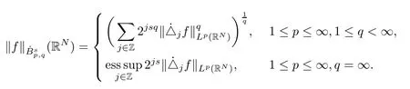
Throughout the paper，without loss of generality，we setμ=μ1=μ2=a=b=¯ρ=1.Before stating our main results，we explain the notations and conventions used throughout.∇lwith an integerl≥0 stands for the any spatial derivatives of orderl.Whenl＜0 orlis not a positive integer，∇lstands for Λldefined by Λsu:=F-1(|ξ|s(ξ))，whereis the Fourier transform ofuand F-1its inverse.We use(s∈R) to denote the homogeneous Sobolev spaces on R3with the normdefined by，Hs(R3) to denote the usual Sobolev spaces with the norm ‖·‖Hs，andLp(1≤p≤∞) to denote the usualLp(R3) spaces with the norm ‖·‖Lp.Finally，we introduce the homogeneous Besov space，lettingbe a cut-offfunction such thatφ(ξ)=1 with|ξ|≤1，and lettingφ(ξ)≤2 with|ξ|≤2.Letψ(ξ)=φ(ξ)-φ(2ξ) andψj(ξ)=ψ(2-jξ) forj∈Z.Then，by the constructionifξ0，we set，so that fors∈R，we define the homogeneous Besov spaces(RN) with the normby

We will employ the notationA≾Bto mean thatA≤CBfor a universal constantC＞0 that only depends on the parameters coming from the problem.For the sake of concision，we write ‖(A，B)‖X:=‖A‖X+‖B‖X.

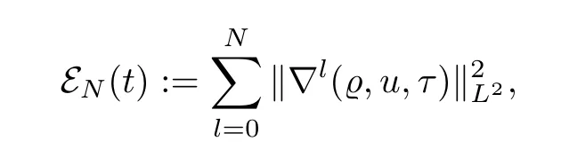
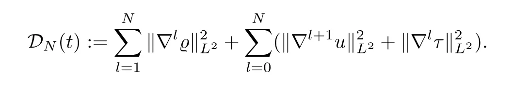
ForN≥3，we define the energy functional by

and the corresponding dissipation rate by

Now，we state our main result about the global existence and decay properties of a solution to the system (1.1)–(1.2) in the following theorems:

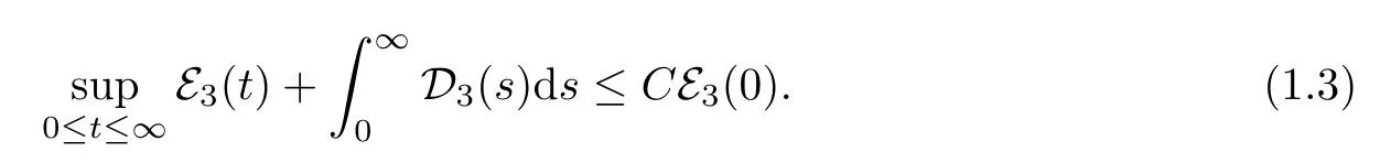
Theorem 1.1LettingN≥3，and assuming that (ρ0-1，u0，τ0)∈HN，there exists a sufficiently smallδ0＞0 such that if E3(0)≤δ0，then the problem (1.1)–(1.2) has a unique global solution (ρ，u，τ)(t) satisfying

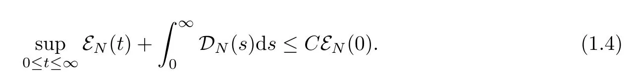
Furthermore，if EN(0)＜∞for anyN≥3，then (1.1)–(1.2) admits a unique solution (ρ，u，τ)(t) satisfying

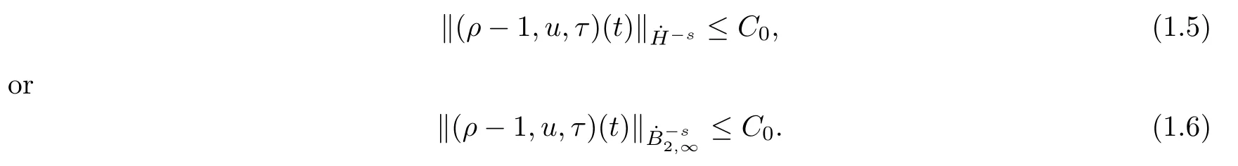
In addition，if the initial data belong to Negative Sobolev or Besov spaces，based on the regularity interpolation method and the results in Theorem 1.1，we can derive some further decay rates of the solution and its higher order spatial derivatives to systems (1.1)–(1.2).

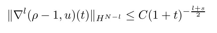
Theorem 1.2Under all the assumptions in Theorem 1.1，let (ρ，u，τ)(t) be the solution to the system (1.1)–(1.2) constructed in Theorem 1.1.Suppose that (ρ0-1，u0，τ0)∈-sfor somesfor somes∈(0，].Then we have

Moreover，fork≥0，ifN≥k+2，it holds that

Note that the Hardy-Littlewood-Sobolev theorem (cf.Lemma 4.4) implies that forp∈This，together with Theorem 1.2，means that theLp-L2type of decay result follows as a corollary.However，the imbedding theorem cannot cover the casep=1;to amend this，Sohinger-Strain[30]instead introduced the homogeneous Besov spacedue to the fact that the endpoint imbeddingholds (Lemma 4.5).At this stage，by Theorem 1.2，we have the following corollary of the usualLp-L2type of decay result:

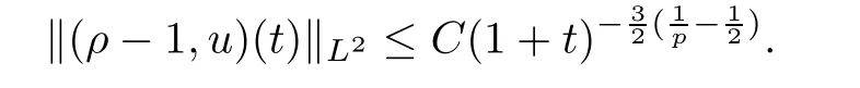
Corollary 1.3Under the assumptions of Theorem 1.2，if we replace theassumption by (ϱ0，u0，τ0)∈Lpfor somep∈[1，2]，then，for any integerk≥0，ifN≥k+2，the following decay result holds:

The rest of our paper is organized as follows:in Section 2，we establish the refined energy estimates for the solution and derive the negative Sobolev and Besov estimates.Furthermore，we use this section to prove Theorem 1.1.Finally，we prove Theorem 1.2 in Section 3.

2 The Global Existence of Solution

In this section，we are going to prove our main result.The proof of local well-posedness for PTT is similar to the Oldroyd-B model (see[7，13])，so we omit the details here.Theorem 1.1 will be proved by combining the local existence of (ϱ，u，τ) to (1.1)–(1.2) and some a priori estimates as well as the communication argument.We first reformulate system (1.1).We setϱ=ρ-1.Then the initial value problem (1.1)–(1.2) can be rewritten as

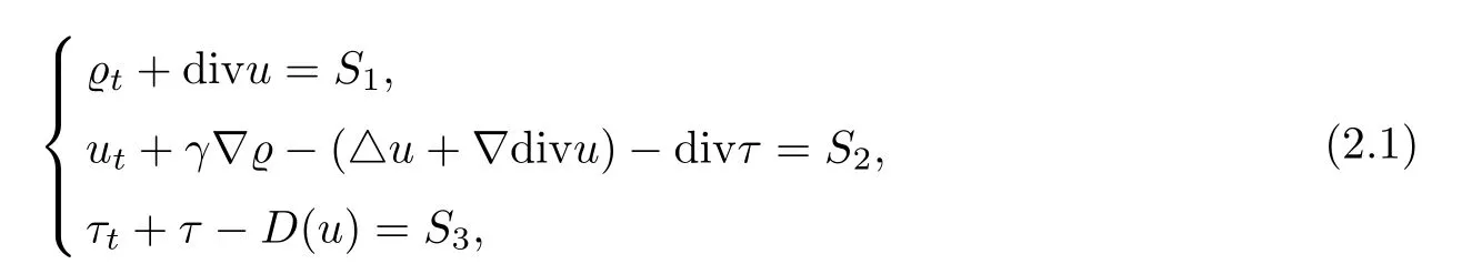
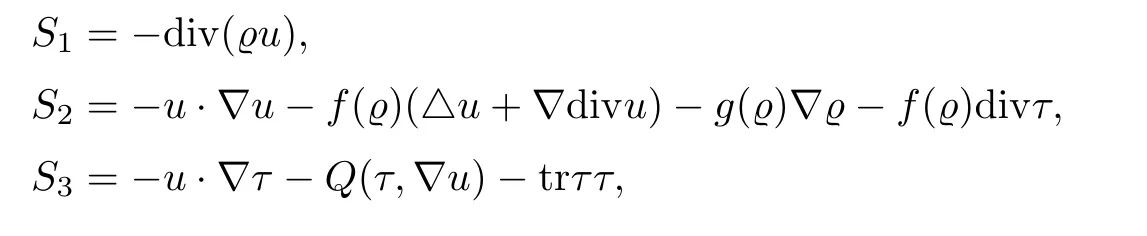
where the nonlinear termsSi(i=1，2，3) are defined as

For simplicity，in what follows，we setp′(1)=1;that isγ=1.

Then，we will derive the nonlinear energy estimates for system (2.1).Hence，we assume that，for sufficiently smallδ＞0，

First of all，by (2.4) and Sobolev’s inequality，we obtain that

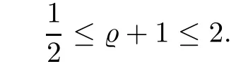
Hence，we immediately have that

2.1 Energy estimates

Before establishing the global existence of the solution under the assumption of (2.4)，we derive the basic energy estimates for the solution to systems (2.1)–(2.2).We begin with the standard energy estimates.

Lemma 2.1If

then，for any integersk≥0 andt≥0，we have that

ProofFor (2.1) onϱ，u，andτ，respectively，we get

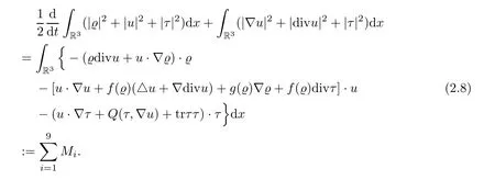
We shall estimate each term on the right hand side of (2.8).First，for the termM1，it is obvious that

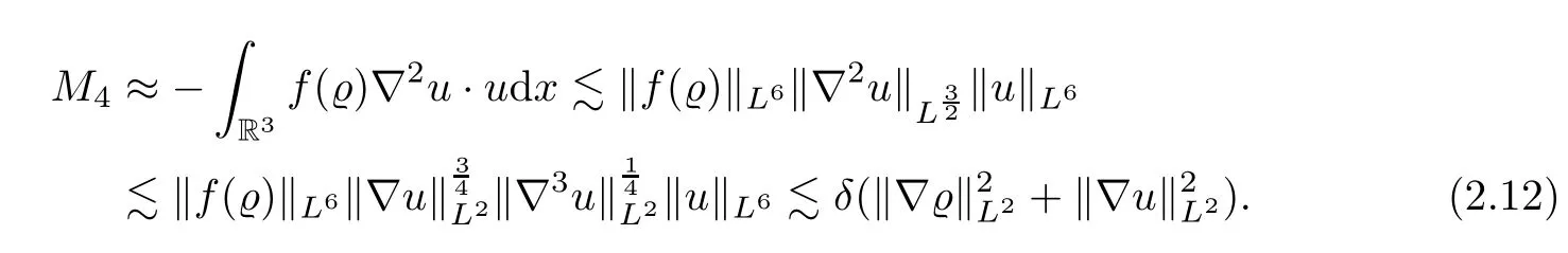
We integrate by parts and by Lemma 4.3 and Hlder’s inequality to get that

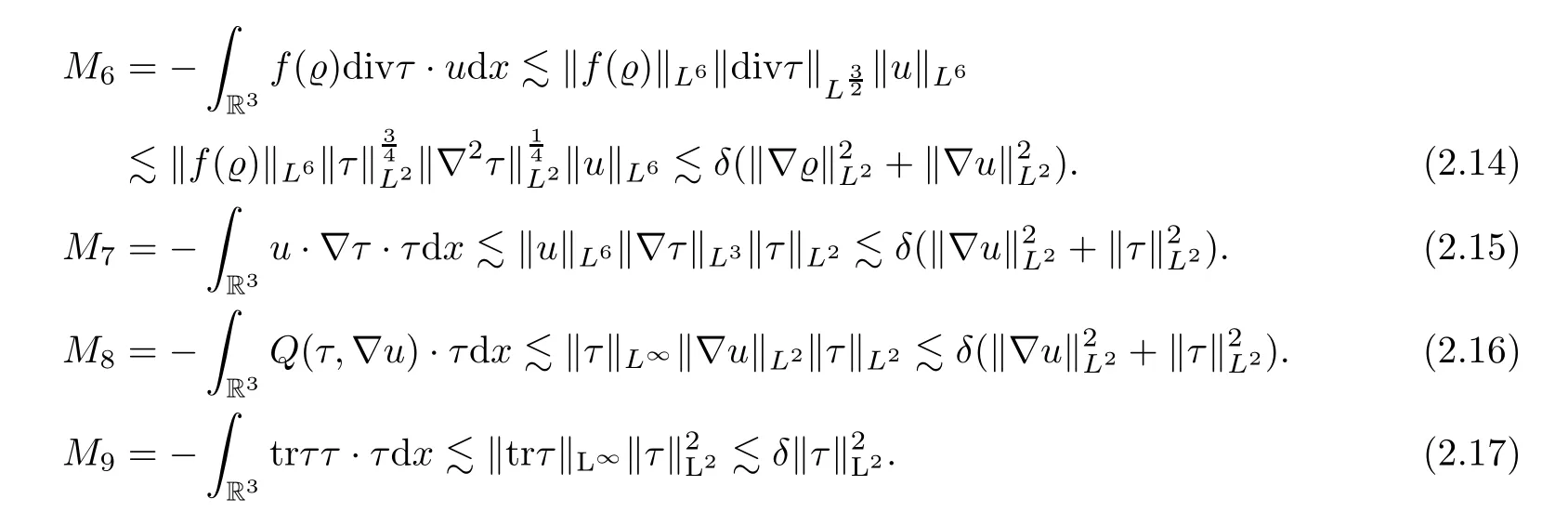
Summing up the estimates forM1–M9，we deduce (2.7)，which yields the desired result. □

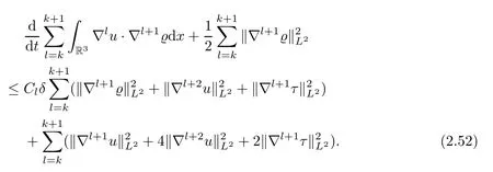
Lemma 2.2Letting all of the assumptions in Lemma 2.1 be in force，for anyk≥0，it holds that

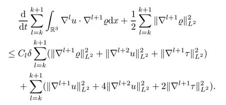
ProofFor any integerk≥0，by the∇l(l=k+1，k+2) energy estimate，for (2.1) onϱ，u，andτ，respectively，we get that

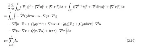
We shall estimate each term on the right hand side of (2.19).First，for the termI1，ifl=1，we further obtain that

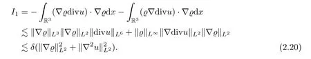
Ifl≥2，then employing the Leibniz formula and by Hlder’s inequality we obtain that

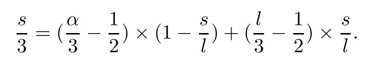
If 0≤s≤[]，by using Lemma 4.1，we estimate the first factor in the above to get that

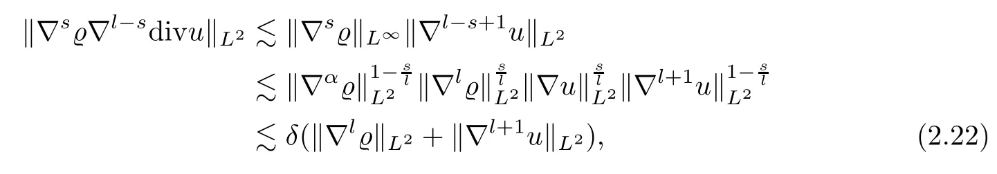
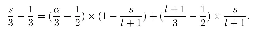
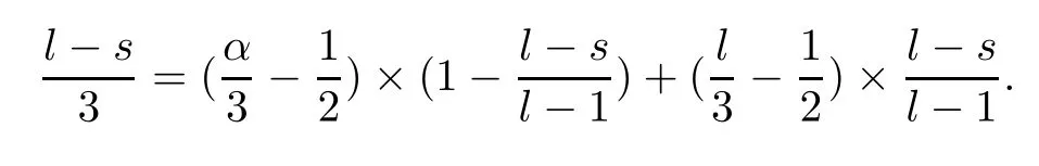
whereαis defined by

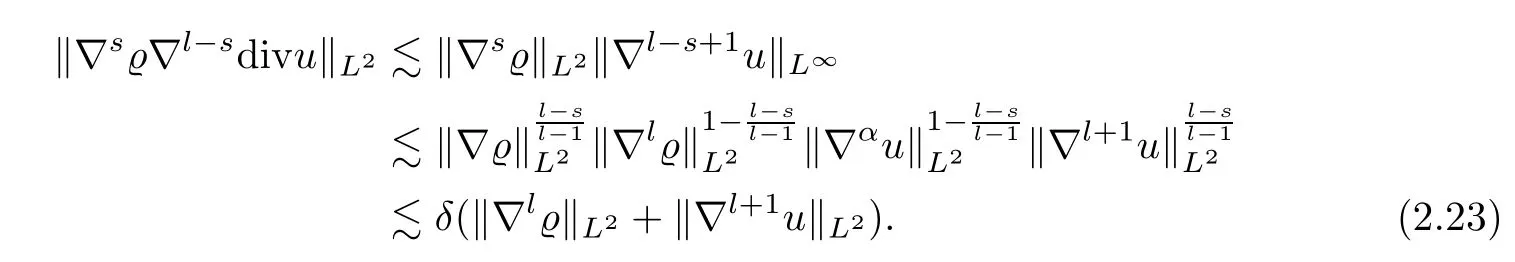
Hereαis defined by

Combining (2.20)–(2.23)，and by Cauchy’s inequality，we deduce that

For the termI2，employing Lemma 4.2，we infer that

For the termI3，

If 0≤s≤[]，by using Lemma 4.1，we estimate the first factor in the above to get that

whereαis defined by

Since 0≤s≤[]，we have that

whereαis defined by

Combining (2.27)–(2.28) and by using Cauchy’s inequality，we deduce that

Now，we estimate the termI4.Ifl=1，we integrate by parts and use Lemma 4.2 and Hlder’s inequality to get that

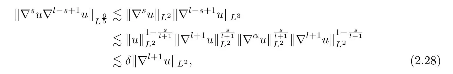
Ifl≥2，we integrate by parts and employ the Leibniz formula and Hlder’s inequality to obtain

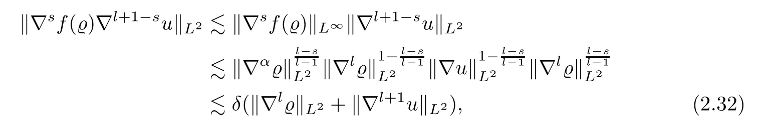
whereαis defined by

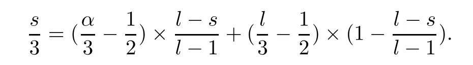
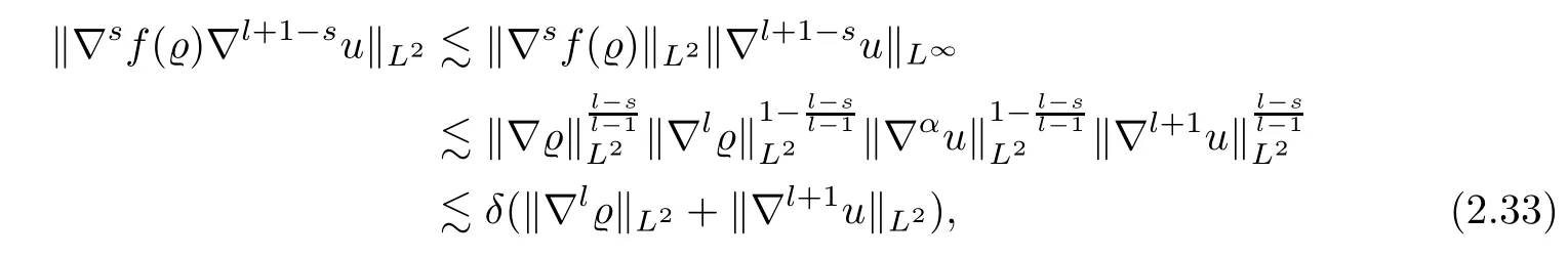
whereαis defined by

Combining (2.30)–(2.33)，we deduce that

Next，we estimate the termI5.Ifl=1，we integrate by parts and use Lemma 4.3 and Hlder’s inequality to get that

Ifl≥2，we integrate by parts to find that

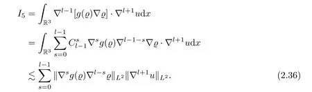
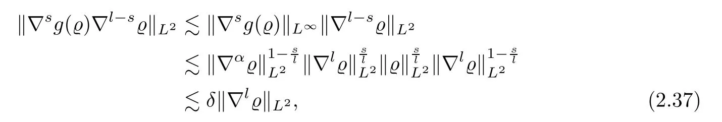
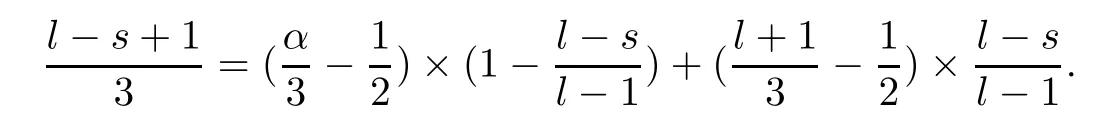
whereαis defined by

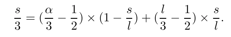
whereαis defined by

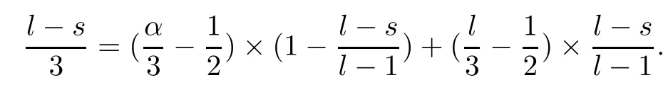
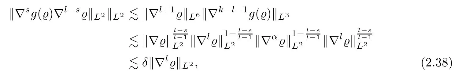
Combining (2.35)–(2.38)，we deduce that

We now estimate the termI6.Ifl=1，by Hlder’s inequality we get that

Ifl≥2，we integrate by parts and employ the Leibniz formula and Hlder’s inequality to obtain that

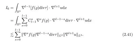
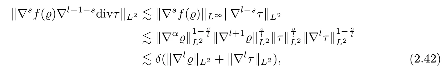
whereαis defined by

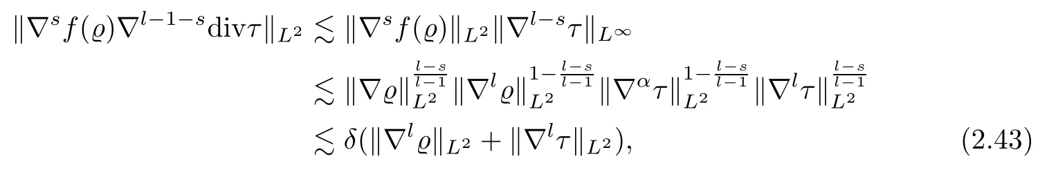
whereαis defined by

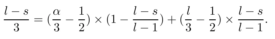
Combining (2.41)–(2.43)，we deduce that

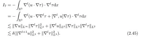
We now estimate the termI7.Using Lemma 4.2 and Hlder’s inequality，we get that

Similarly toI1，we can bound

We now estimate the termI9.Ifl=1，we further obtain that

Ifl≥2，by Hlder’s inequality，we get that

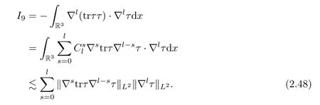
If 0≤s≤[]，by using Lemma 4.1，we estimate the first factor in the above to get that

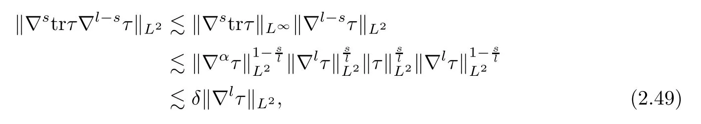
whereαis defined by

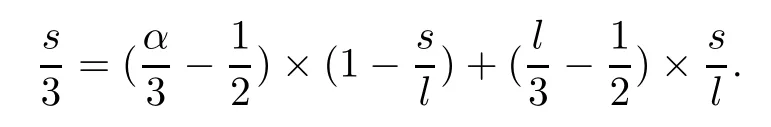
Since 0≤s≤[]，we have that

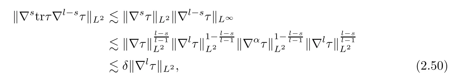
whereαis defined by

Combining (2.47)–(2.50)，we deduce that

Summing up the estimates forI1–I9，i.e.，(2.24)，(2.25)，(2.29)，(2.34)，(2.39)，(2.44)，(2.45)，(2.46) and (2.51)，we deduce (2.18)，which yields the desired result. □

We now recover the dissipative estimates ofϱby constructing some interactive energy functionals in the following lemma:

Lemma 2.3Let all of the assumptions in Lemma 2.1 be in force.Then，for anyk≥0，it holds that

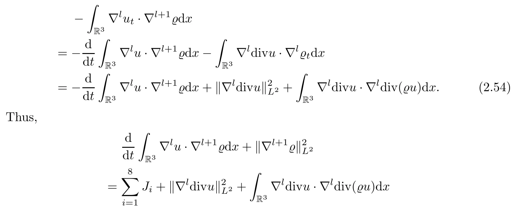
ProofApplying∇l(l=k，k+1) to (2.1)2，multiplying∇l+1ϱ，and integrating by parts，we get that

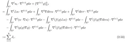
For the first term on the left-hand side of (2.53)，by (2.1)1and integrating by parts for both thet-andx-variables，we may estimate

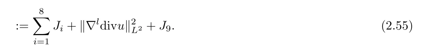
Now，we concentrate our attention on estimating the termsJ1–J9. First，employing Cauchy’s inequality，it holds that

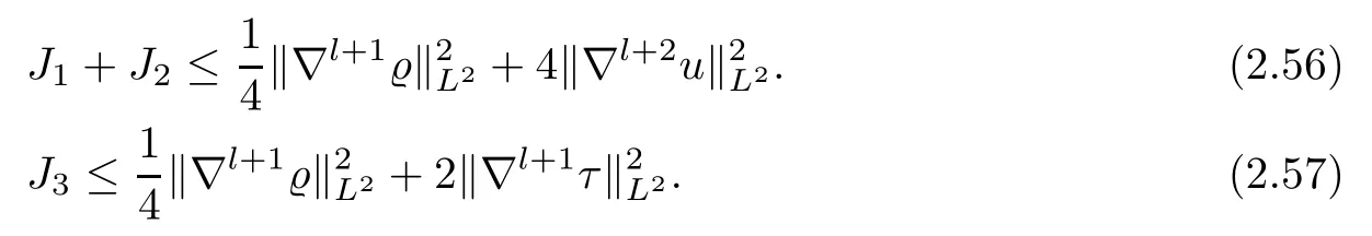
Moreover，taking into account (2.27)–(2.28)，we are in a position to obtain that

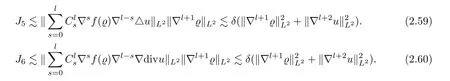
Similarly to (2.30)–(2.33)，using Hlder’s inequality，Lemma 4.1 and Lemma 4.3，the termsJ5，J6can be estimated as follows:

Furthermore，taking into account (2.35)–(2.38)，applying Hlder’s inequality，Lemma 4.1 and Lemma 4.3，we obtain that

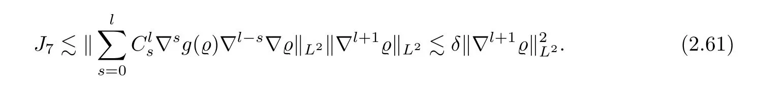
Similarly to the estimates of (2.42)–(2.43)，we further obtain that

Finally，similarly toI9，by integration by parts and Lemma 4.1，we get that

Putting these estimates into (2.55)，and summing up withl=k，k+1，we finally obtain that

Thus，we have completed the proof of Lemma 2.2. □

2.2 Negative Sobolev estimates

In this subsection，we will derive the evolution of the negative Sobolev norms and Besov norms of the solution.In order to estimate the nonlinear terms，we need to restrict ourselves to the fact thatFirst，for the homogeneous Sobolev space，we will establish the following lemma:

Lemma 2.4Fors，we have that

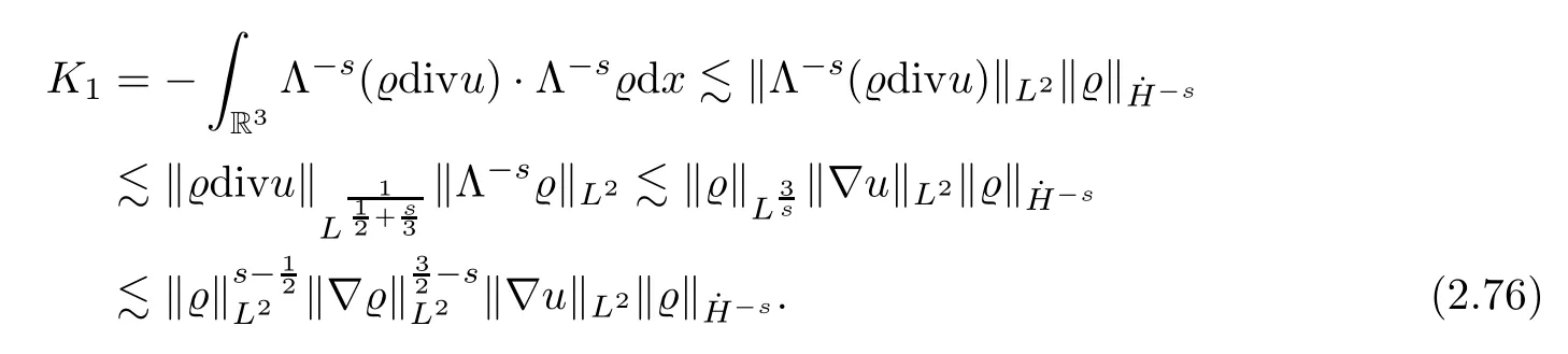
ProofApplying Λ-sto (2.1)，and multiplying the resulting identities by Λ-sϱ，Λ-suand Λ-sτ，respectively，summing up them and then integrating over R3by parts，we get that

IfsThen，using Lemma 4.4，together with Hlder’s and Young’s inequalities，we obtain that

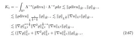
Similarly，we can bound the termsK2–K5by

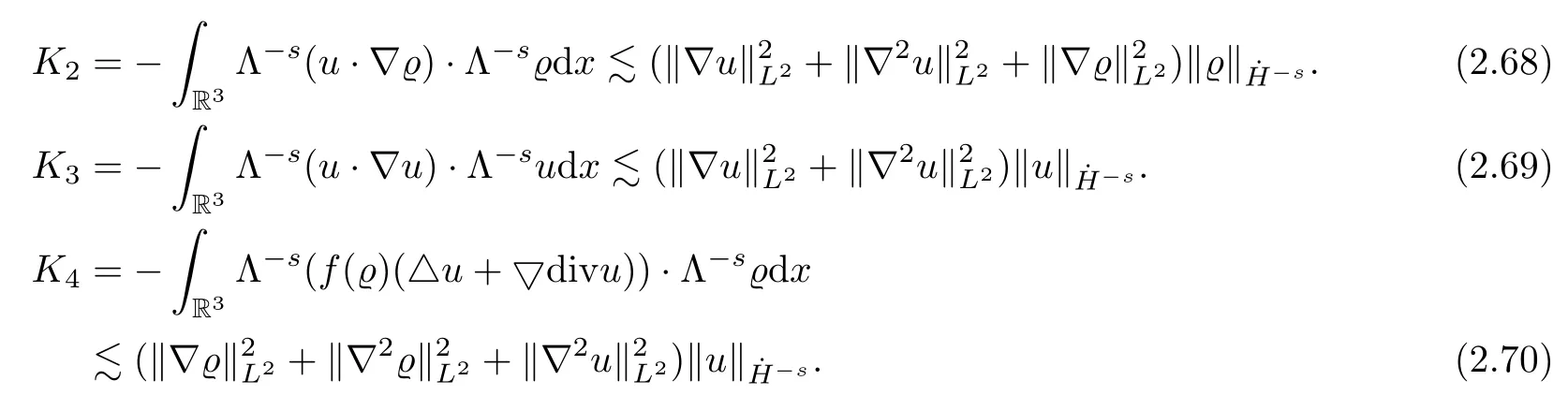
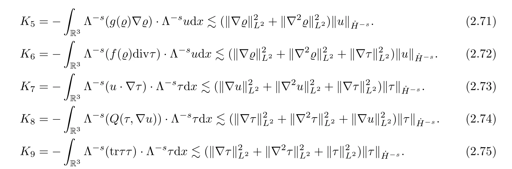
Hence，plugging the estimates (2.67)–(2.75) into (2.66)，we deduce (2.64).

Now ifswe shall estimate the right-hand side of (2.66) in a different way.Sinces∈，we have thatThen，by Lemmas 4.5 and 4.1，we obtain that

Similarly，we can bound the remaining terms by

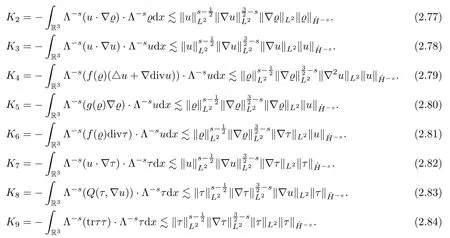
Hence，plugging estimates (2.76)–(2.84) into (2.66)，we deduce (2.65). □

2.3 Negative Besov estimates

We replace the homogeneous Sobolev space by the homogeneous Besov space.Now，we will derive the evolution of the negative Besov norms of the solution (ϱ，u，τ) to (2.1)–(2.2).More precisely，we have

Lemma 2.5Let all of the assumptions in Lemma 2.1 hold.Then，fors∈(0，]，we have that

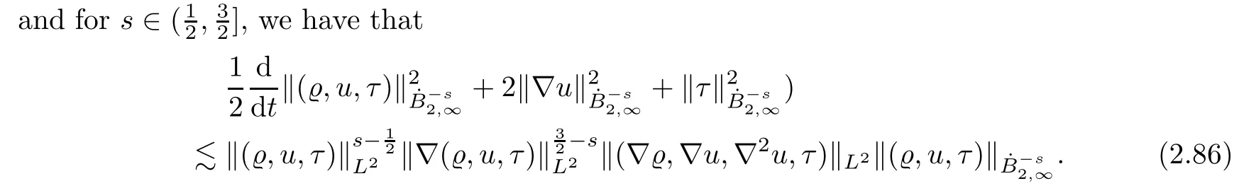
ProofApplying thejenergy estimate of (2.1) with a multiplication of 2-2sjand then taking the supremum overj∈Z，we infer that

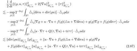
According to Lemma 4.5 and (2.87)，the remaining proof of Lemma 2.5 is exactly the same with the proof of Lemma 2.4，except that we allow thats=and replace Lemma 4.4 with Lemma 4.5，and the-snorm by thenorm. □

Next，we will combine all the energy estimates that we have derived in order to prove Theorem 1.1;the key point here is that we only assume that theH3norm of initial data is small.

ProofWe first close the energy estimates at theH3-level by assuming thatpE3(t)≤δis sufficiently small.From Lemma 2.2，takingk=0，1 in (2.18) and summing up，we deduce that，for anyt∈[0，T]，

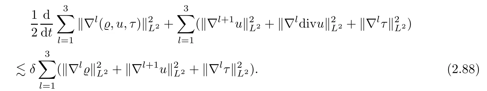
From this，together with Lemma 2.1，we deduce that，for anyt∈[0，T]，

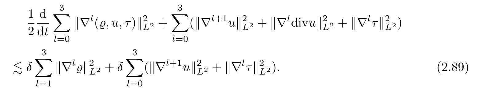
In addition，taking thek=0，1 in (2.52) of Lemma 2.3 and summing up，we obtain that

Taking into account the smallness ofδ，by a linear combination of (2.89) and (2.90)，we deduce that there exists an instant energy functional～E3(t) equivalent to E3(t) such that

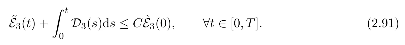
By a standard continuity argument，we then close the a priori estimates if we assume，at the initial time，that(0)≤δ0is sufficiently small.This concludes the unique global smallsolution.

From the global existence of thesolution，we shall deduce the global existence of theNsolution.ForN≥3，t∈[0，∞]，applying Lemma 2.2 and takingk=0，1，...，N-2，we infer that

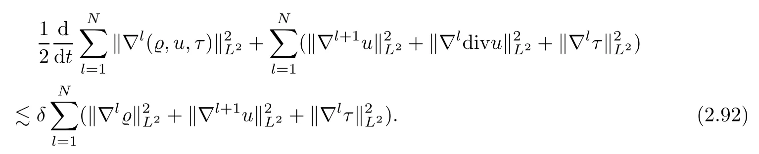
From this，together with Lemma 2.1，we deduce that

Furthermore，by Lemma 2.3，and takingk=0，1，...，N-2，we have that

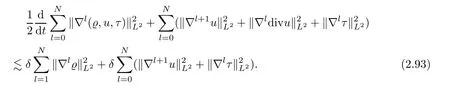
By a linear combination of (2.93) and (2.94)，we infer that there exists an instant energy functionalN(t) taht is equivalent to EN(t) such that

3 Convergence Rate of the Solution

Having in hand the conclusion of Theorem 1.1，Lemma 2.4 and Lemma 2.5，we now proceed to prove the various time decay rates of the unique global solution to (2.1)–(2.2).

Proof of Theorem 1.2In what follows，for convenience of presentation，we define a family of energy functionals and the corresponding dissipation rates as

Taking into accounts Lemmas 2.1–2.3，we have that，fork-0，1，...，N-2，

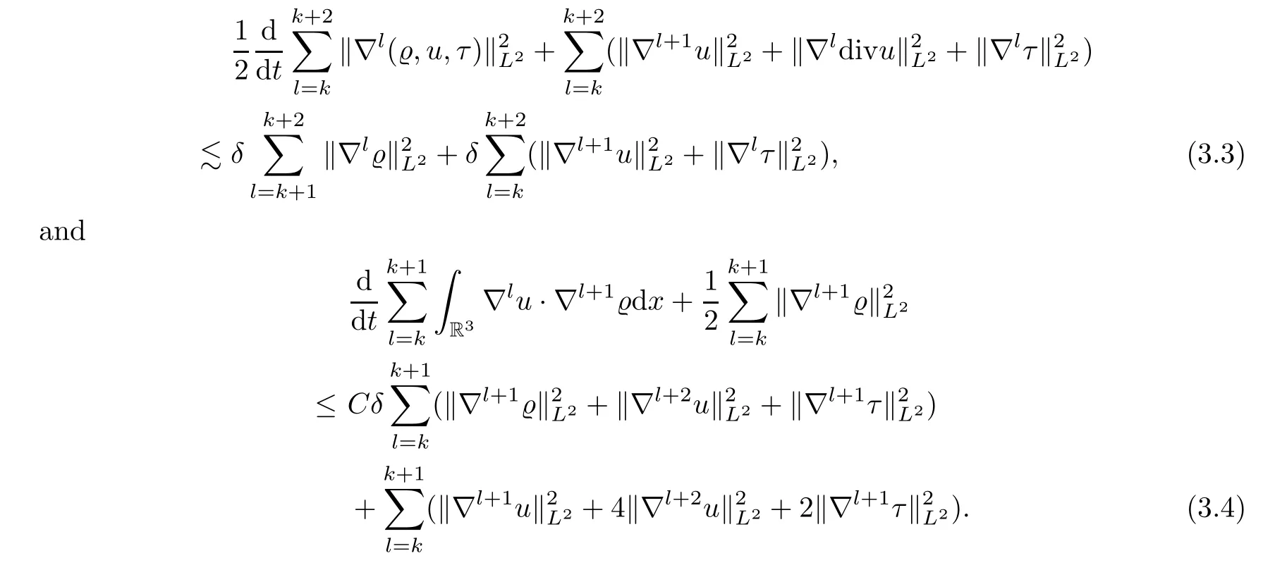
By a linear combination of (3.3) and (3.4)，sinceδis small，we deduce that there exists an instant energy functionalthat is equivalent tosuch that

Similarly，applying Lemma 4.7，fors＞0 andk+s≥0，we have that

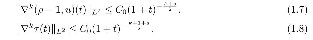
As a consequence，from (3.6)–(3.7)，it follows that

This proves the decay (1.7).Regarding (1.8)，applying∇kto (2.1)3and multiplying the resulting identity by∇kτ，then integrating over R3，we have that

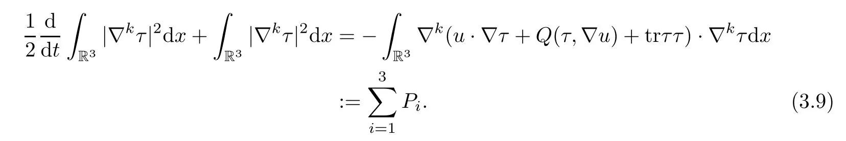
For the termP1，similarly as toI7，using (1.7)，we deduce that

Similarly as forP1，the termP2can be estimated as

For the termP3，similarly as toI9，we deduce that

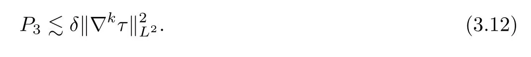
Combining (3.10)–(3.12)，we deduce from (3.9) that

This，together with Gronwall’s inequality，implies (1.8).

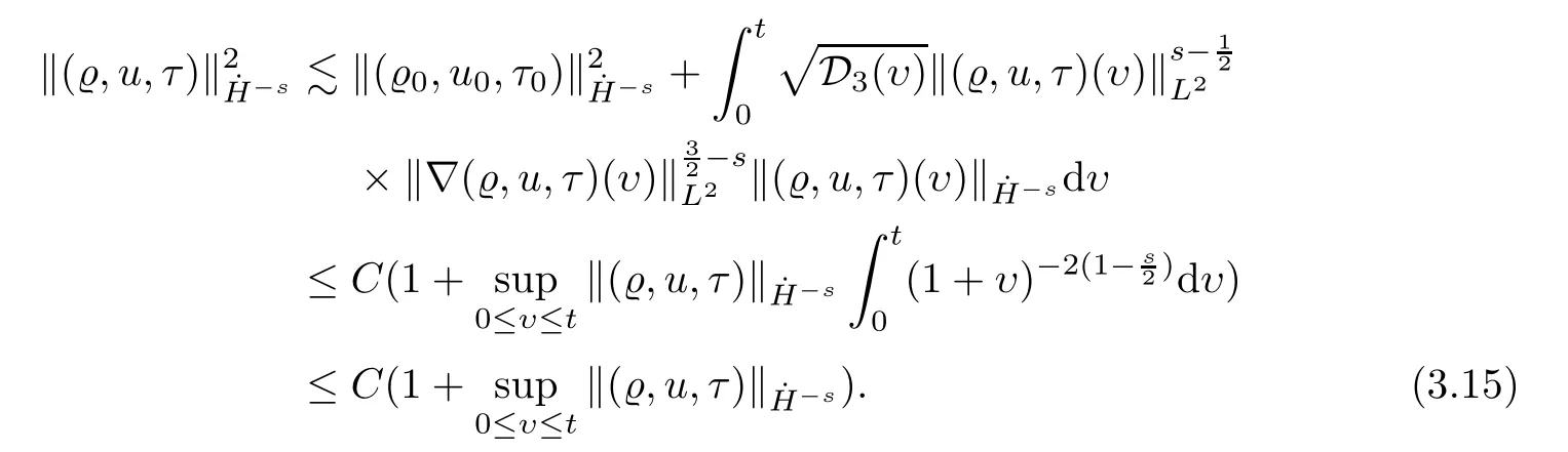
Finally，we turn back to the proof of (1.5) and (1.6).First，we propose to prove (1.5) by Lemma 2.4.However，we are not able to prove it for allsat this moment，so we must distinguish the argument by the value ofs.First，this is trivial for the cases=0，then，fors，integrating (2.64) in time，and by (1.3)，we obtain that

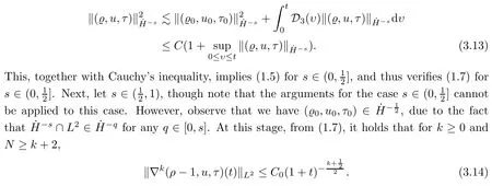
Thus，integrating (2.65) in time fors∈(，1) and applying (3.14) yields that

In the last inequality，we used the fact thats∈(，1)，so the time integral is finite.By Cauchy’s inequality，this implies (1.5) fors∈(，1).From this，we also verify (1.7) fors∈(，1).Finally，lettings∈[1，)，we chooses0such thats-＜s0＜1.Then (ϱ0，u0，τ0)∈-s0，and from (1.7)，it holds that

fork≥0 andN≥k+2.Therefore，similarly to (3.15)，using (3.16) and (2.65) fors∈(1，)，we conclude that

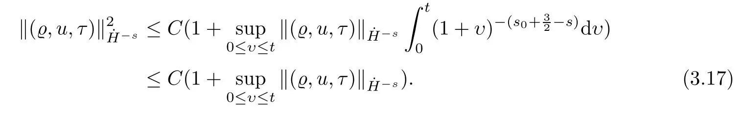
Here，we have taken into account the fact that，so the time integral in (3.17) is finite.This implies (3.14) for，and thus we have proved (1.7) for.The rest of the proof is exactly same as above;we only need to replace Lemma 4.6 and Lemma 2.4 by Lemma 4.7 and Lemma 2.5，respectively.Then we can deduce (1.6) fors.For the sake of brevity，we omit the details here.Thus，we have completed the proof of Theorem 1.2. □

4 Appendix:Analysis Tools

In this subsection we collect some auxiliary results.First，we will extensively use the Sobolev interpolation of the Gagliardo-Nirenberg inequality.

Lemma 4.1([24]) Letting 0≤m，α≤l，we have that

where 0≤θ≤1 andαsatisfies that

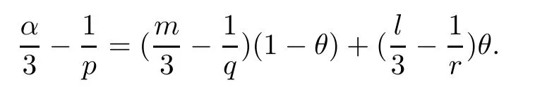
Here，whenp=∞，we require that 0＜θ＜1.

We recall the following commutator estimate:

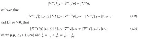
Lemma 4.2([15]) Lettingm≥1 be an integer and defining the commutator

We now recall the following elementary but useful inequality:

Lemma 4.3([36]) Assume that ‖ϱ‖L∞≤1 andp＞1.Letg(ϱ) be a smooth function ofϱwith bounded derivatives of any order.Then，for any integerm≥1，we have that

Ifs∈[0，)，the Hardy-Littlewood-Sobolev theorem implies the followingLptype inequality:

Lemma 4.4([31]) Let.Then

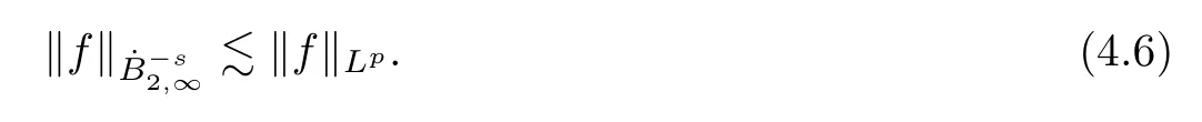
In addition，fors∈(0，]，we will use the following result:

Lemma 4.5([12]) Let.Then，

We will employ the following special Sobolev interpolation:

Lemma 4.6([37]) Lettings≥0 andl≥0，we have that

Lemma 4.7([30]) Lettings≥0 andl≥0，we have that