Depth estimation using an improved stereo network*

Wanpeng XU ,Ling ZOU‡ ,Lingda WU ,Yue QI ,Zhaoyong QIAN

1Science and Technology on Complex Electronic System Simulation Laboratory,Space Engineering University,Beijing 101416,China

2Peng Cheng Laboratory,Shenzhen 518055,China

3Digital Media School,Beijing Film Academy,Beijing 100088,China

†E-mail:xuwp@pcl.ac.cn;zouling@bfa.edu.cn

Abstract: Self-supervised depth estimation approaches present excellent results that are comparable to those of the fully supervised approaches,by employing view synthesis between the target and reference images in the training data.ResNet,which serves as a backbone network,has some structural deficiencies when applied to downstream fields,because its original purpose was to cope with classification problems.The low-texture area also deteriorates the performance.To address these problems,we propose a set of improvements that lead to superior predictions.First,we boost the information flow in the network and improve the ability to learn spatial structures by improving the network structures.Second,we use a binary mask to remove the pixels in low-texture areas between the target and reference images to more accurately reconstruct the image.Finally,we input the target and reference images randomly to expand the dataset and pre-train it on ImageNet,so that the model obtains a favorable general feature representation.We demonstrate state-of-the-art performance on an Eigen split of the KITTI driving dataset using stereo pairs.

Key words: Monocular depth estimation;Self-supervised;Image reconstruction

1 Introduction

The technology for obtaining accurate and dense depth maps from two-dimensional (2D) images is a valuable and fundamental task that has extensive applications in three-dimensional (3D) reconstruction,augmented reality (Newcombe et al.,2011),mapping and localization,robotics navigation (Desouza and Kak,2002),and autonomous driving(Menze and Geiger,2015).The traditional approaches to gaining depth have relied mainly on the assumption that multiple perspectives are available,including binocular,multi-view stereo,shape-from-X,and structure from motion,but the high computational complexity of traditional approaches affects the matching effect,especially for low-texture scenes.

Depth estimation approaches based on active sensing,such as laser imaging detection and ranging(LIDAR),structured light projection,and time-offlight (TOF) measurement,obtain accurate depth information directly.Although these sensors have high accuracy,they still have shortcomings.For instance,the LIDAR sensor is expensive and can obtain only sparse depth maps.The TOF camera can be used only for indoor scenes and to obtain depth information for short distances.

Ordinary cameras are widely used due to their high resolution and low price.With the enhancement of deep learning in the field of geometry,researchers automatically infer high-quality color depth maps from monocular input images,and remarkable results have been achieved using images paired with depth maps as the input.Obtaining a lot of depth annotations is costly and time-consuming,so it limits the application of such methods.

As an alternative,self-supervised methods,which exploit view synthesis in the training data using monocular sequences (Zhou TH et al.,2017)or stereo pairs (Godard et al.,2017),have shown promising results,even compared to the methods that are supervised with ground-truth depth.

However,ResNet,which was designed for classification cases,is employed by the best practice as the backbone network,but it has some structural defects when applied to the downstream field.For instance,the network reception field is too small to cope with dynamic scenes and occlusion.Consequently,the downstream applications adopt a series of improvements such as using pyramid representation to increase the size of the receiving field,adding masks to handle occlusion,and using more expensive“spatial attention.”Inspired by He et al.(2016a)and Duta et al.(2020),we embrace the improved information flow propagation and learning space features,to build a new depth estimation backbone network.

No pixels that violate camera motion assumptions are traditionally expected when using stereo pairs as the input for self-supervised methods.However,the low-texture area deteriorates the performance.We exploit an auto-masking loss to ignore those pixels and to improve the accuracy of depth estimation.Fig.1 shows a single image and the depth estimation outcome of our model.

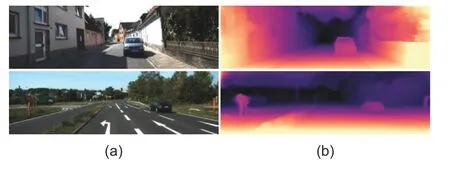
Fig.1 Our depth prediction results on the KITTI dataset using Eigen split:(a) original images;(b)depth maps predicted by our models

Our main contributions are as follows:(1) An improved network architecture that performs selfsupervised monocular depth estimation using stereo pairs is proposed to better propagate information through the network’s layers.(2) A novel disparity consistency loss ignores the training pixels of images in the low-texture area.Together,these improvements produce scores that outperform selfsupervised methods using rectified stereo pairs on the KITTI dataset(Eigen and Fergus,2015).Fig.2 shows our overall consideration.

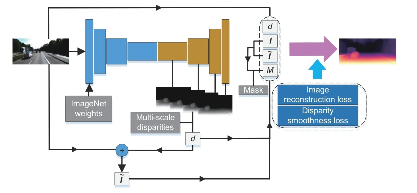
Fig.2 Illustration of our deep estimation model architecture

2 Related works

Here,we review the literature relevant to the monocular depth estimation.Related works are divided into supervised methods (which supervise training using ground-truth depth) and selfsupervised approaches(which supervise training using the internal relationships of the data).

2.1 Supervised methods

Without a second image for triangulation,depth estimation seems to be an ill-posed problem since a single image can project to multiple plausible depths.In response to this problem,learning-based methods have demonstrated the powerful ability to fit predictive models taking images paired with depth maps as the input.

Eigen et al.(2014) proposed a two-scale deep neural network.The coarse network was used to predict the overall information,and the fine network was used to optimize local information.Eigen and Fergus (2015) changed the prediction of depth information only to the simultaneous prediction of depth,normal,and label.Laina et al.(2016) removed the fully connected layer directly,using a structure similar to the pre-trained network structure instead.The entire network was regarded as an encoder-decoder process.Other algorithms,in the form of combining non-parametric scene sampling (Karsch et al.,2012),local predictions (Saxena et al.,2009),and end-to-end supervised learning(Eigen et al.,2014),have been explored.Optical flow (Wang Y et al.,2018) and stereo estimation(Kendall et al.,2017;Ummenhofer et al.,2017)have the best results among learning-based approaches.Recently,a growing number of researchers have employed weakly supervised training data,including sparse ordinal depths (Zoran et al.,2015;Chen WF et al.,2016),known object sizes (Wu et al.,2018),unpaired synthetic depth data(Atapour-Abarghouei and Breckon,2018;Zou et al.,2018),or supervised appearance matching terms (Zhan et al.,2018).All these approaches still need to collect other annotations or additional depth maps.

Synthesizing training data is an alternative method (Mayer et al.,2018).It is hard to generate photorealistic synthetic images because a domain gap exists between synthetic and real images.Furthermore,it is not easy to produce large amounts of synthetic data that include different real-world appearances and movements.Due to their fully supervised nature,the above methods require ground truth during training,but it is not realistic to obtain ground truth in various environments.

2.2 Self-supervised methods

Learning to predict depth without labels is a powerful concept,thanks to the geometrical relationships between multiple captures of the same scene.As an alternative,self-supervised monocular depth estimation methods train models using image reconstruction as the supervisory signal,which exploits the monocular sequence or stereo pairs as the input.

2.2.1 Stereo depth estimation

Žbontar and LeCun(2016)first trained the convolutional neural network using stereo pairs to displace the matching cost calculation.Various approaches have produced results superior to those of fully supervised methods.Garg et al.(2016) predicted continuous disparity values;Xie et al.(2016)used the discrete depth model to tackle the multiview synthesis;Luo WJ et al.(2016) treated this task as a multi-class classification problem;Godard et al.(2017) increased the left-right depth consistency constraint.Stereo-based algorithms have been extended with generative adversarial networks (Luo WJ et al.,2016) and semi-supervised data (Kuznietsov et al.,2017),and for real-time use(Poggi et al.,2018).Recently,Watson et al.(2019)explored semiglobal matching(SGM)as additional supervision for the single image depth estimation task,achieving excellent results.

2.2.2 Monocular depth estimation

The other method is to exploit monocular video for training with adjacent frames as supervisory signals.Although this method has fewer restrictions,it must estimate the pose between adjacent frames while estimating the depth.Performance may be deteriorated when there is object motion in the scene.

SfMLearner fulfills a pioneering achievement(Zhou TH et al.,2017) for this work,training the depth estimation network and pose estimation network separately.This manner was boosted by employing multi-task learning (Zou et al.,2018),point-cloud alignment(Mahjourian et al.,2018),and differentiable direct visual odometry (DVO) (Luo CX et al.,2020).Multiple motion masks (Vijayanarasimhan et al.,2017)were also employed to train a sophisticated model.To handle moving objects,optical flow was used to explain the moving object(Zhan et al.,2018).Casser et al.(2019)and Gordon et al.(2019) employed segmentation masks to handle potential moving objects.Aleotti et al.(2018)proposed a generative adversarial network model to tackle the monocular scenario.Three-dimensional consistency was considered in Chen YH et al.(2019).A minimum reprojection loss was proposed by Godard et al.(2019) in response to occlusion using auto-masking loss.Guizilini et al.(2020)exploited a 3D convolution module to save the spatial structure.Zhou LP and Kaess (2020) proposed a new visual odometry method,which uses structural rules in the artificial environment.

3 Methods

In this section,we describe our improved monocular depth estimation network architecture in detail.It is designed to infer the depth maps more precisely from a single image in a self-supervised manner.In addition,we introduce the loss function based on the binary mask and ignore low-texture pixels between the stereo pairs.Finally,we expand the dataset by randomly inputting the left and right images.

3.1 Network architecture

Although the efficiency and effectiveness of depth estimation are greatly improved,it is a better practice to use ResNet as the basis of transfer learning.ResNet is designed for classification instances.In most cases,it has some structural flaws when applied to downstream domains.For example,the receptive field of the network is too small to tackle occlusion and moving objects.In response to this situation,and inspired by He et al.(2016a)and Duta et al.(2020),we improve information flow through the network and boost the ability to acquire spatial information.

3.1.1 Improved information flow through the network

He et al.(2016a)stacked several residual building blocks(ResBlocks),as shown on the left in Fig.3.The ResBlock is composed of one 3×3 convolutional layer,two 1×1 convolutional layers,three batch normalization(BN)layers,and three rectified linear unit(ReLU) layers.However,at the end of each Res-Block bottleneck,there is a ReLU,which may have an unfavorable effect on the spread of information by zeroing the negative signal that may also be an important weight for backpropagation.This drawback had been overcome in He et al.(2016b) by getting rid of the last ReLU amid each ResBlock bottleneck.

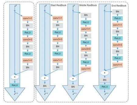
Fig.3 Improved ResBlocks:ResNet ResBlocks (left) and our approach (right)

Leaving the main path completely free when allowing feature maps to pass the network in an uncontrolled way will create two main dilemmas.First,there are no BN layers after addition.Thus,with the continuous stacking of blocks,the final signal will become increasingly“non-standard”and cause learning to be difficult.Second,without any nonlinear mechanism in the main path,the learning capability will be limited.Given these two problems,to stabilize the signal,we employ the approach proposed in Duta et al.(2020)to ensure that each stage has only one nonlinear mechanism,which is placed after a BN layer at the end of the ResBlock.

Here we take only 50 layers as an example on the right of Fig.3,although this can be extended to any depth.For the case with 50 layers,the framework has three ResBlocks in stage 1,four in stage 2,six in stage 3,and three in stage 4.Each stage includes three types:(1)One Start ResBlock adjusting the number of channels to align the projection shortcut;(2) One End ResBlock,followed by a BN and a ReLU,preparing and stabilizing the signal into the next stage;(3)Any number of Middle ResBlocks(the corresponding stage for the case with 50 layers has[1,2,4,1]Middle ResBlocks),as shown in Fig.4.Unlike ResNet,in our method,only four ReLUs on the main propagation path can retain as many effective backpropagation nodes as possible while maintaining the model’s learning ability.

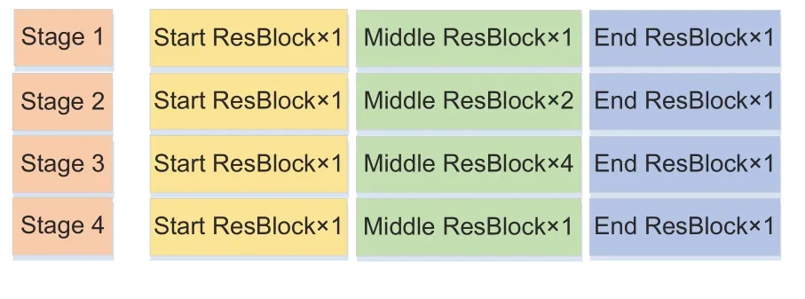
Fig.4 Construction of each main stage

3.1.2 Improved projection shortcut

As we can see in Fig.5a,the projection shortcut in ResNet is applied to feature maps to make element-wise addition,where the channels of feature maps do not match the output.When the stride of convolution is set to align the output space size,it will skip 75% of the feature maps,which will result in significant information loss.However,the remaining 25% of the feature maps are randomly selected by conv1×1,and there is no clear standard.When the output of the projection shortcut is added to the main path,the noisy output,which contributes half of the information,injures the information flow.

Our projection shortcut is presented in Fig.5b.To select the highest activation,we design a spatial projection mapping that consists of a 3×3 maxpooling layer whose stride is 2,a conv1×1 with stride 1,and a BN layer.To ensure element-wise addition on the same spatial window,the kernel size of the max-pooling is consistent with the conv3×3 of the ResBlock.In addition to reducing information loss and signal disturbance,the spatial projection helps preserve spatial structure information.

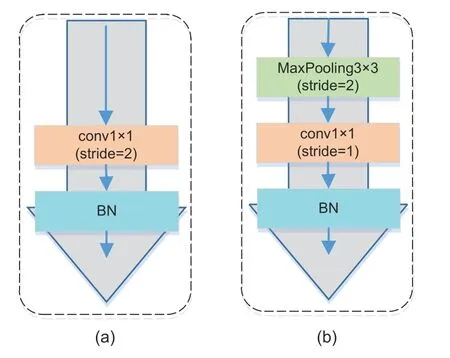
Fig.5 Improved projection shortcut:(a) ResNet projection shortcut;(b) our projection shortcut

We add only a max-pooling layer in each projection shortcut stage.For a network with dozens of layers,the added parameters and calculations are negligible.In contrast,there are only four ReLUs on the backbone path.With the increase of the network depth,the spread of information is smoother than ResNet,and it takes 79 hours,which is 2 hours fewer than ResNet with the same training parameters.We will show the training parameters in Section 4.1.

3.1.3 Grouped building block

The bottleneck in ResNet includes two conv1×1 layers,playing the role of controlling the number of channels.One conv3×3 layer shoulders the responsibility of learning spatial features.To keep the computational cost under control,the conv3×3 is allocated the smallest number of channels,as shown in Fig.6a.This approach limits the ability of the model to learn spatial features.

In our bottleneck,the feature map with the largest number of channels has been assigned to the conv3×3.We embrace grouped convolution to perform the convolution operation independently for each group.This manner can improve accuracy while reducing floating-point operations.Inspired by Duta et al.(2020),the conv3×3 acquires the maximum number of channels,as shown in Fig.6b.

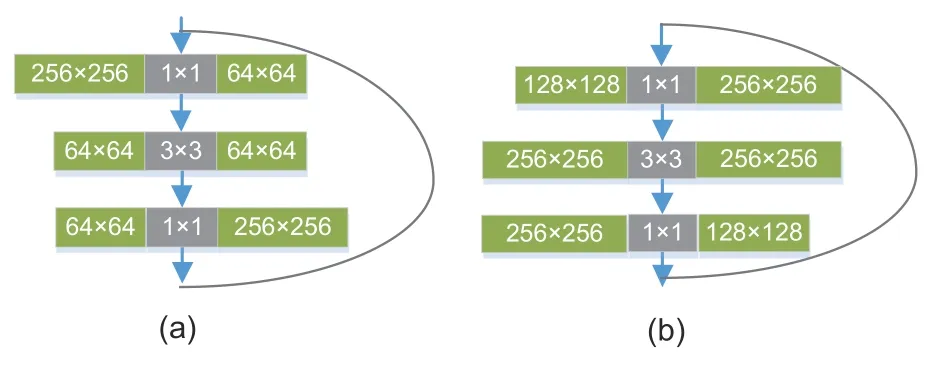
Fig.6 Improved bottleneck numbers:(a) ResNet bottleneck numbers;(b) our bottleneck numbers

3.2 Training loss

There is no need to consider static frames and non-rigid motion in the training data when employing the rectified stereo pairs as the input for training.However,in low-texture areas,the camera motion assumptions will still be broken down,and performance may be deteriorated.During testing,the pixels in the low-texture area will be projected to infinity,and holes will appear there.To train our improved deep estimation network architecture,we obtain the final training loss as

wheresdenotes the sampling round(the feature size,i.e.,the resolution,will be reduced by half in turn).The total loss must be added up on all scales.In this study,we use four different resolutions to estimate the depth.

We define the scale lossLs(s=1,2,3,or 4),a sum of two main contributions at each scale:

whereLpis the appearance matching loss,Lsmoothis a smoothness term,Mpis a binary mask,andλis a hyper-parameter.The left or right image is fed into the convolutional neural network randomly for calculation.

1.Appearance matching loss

Depth estimation is treated as one kind of novel view synthesis.During training,the network predicts the appearance of the original image by sampling pixels from the opposite viewpoint of stereo pairs.Because it is completely differentiable,we use a bilinear sampling method that is based on the spatial transformer network (STN) (Jaderberg et al.,2015)to sample the input image.Following Godard et al.(2017),we use L1 and structural similarity measure(SSIM)(Wang Z et al.,2004) to encode our reconstructed image based on the target image:

whereNis the number of pixels,Idenotes the original image,ˆImeans the reconstructed image,andα0.85 in training.

Inspired by Godard et al.(2019),using a binary mask,we can filter out the pixels whose appearance does not change between the stereo pairs.This method can eliminate the effect of pixels in a low-texture region in the network.If there are no relatively static pixels,the error between the warped image and the original image must be smaller than the error between the left and right images:

whereIlandIrmean the left and right images in the stereo pair,respectively.We show experimentally that this mask can bring significant improvements for a test result.

2.Disparity smoothness loss

For the sake of regularizing the disparity maps in low-image gradient areas,an edge-aware term(Eq.(5)) is incorporated.This cost enforces the predicted disparity with an L1 penalty on the disparity gradient∂d.We also weight the cost with an edge-aware term using the image gradient∂I.

where∂xdindicates the disparity gradient in thexdirection,∂ydindicates the disparity gradient in theydirection,∂xIindicates the image gradient in thexdirection,and∂yIindicates the image gradient in theydirection.

3.3 Implementation details

We introduce three improvements to the depth estimation backbone network.First,we adjust the structure of ResBlocks to change the number of activation functions,which achieves the purpose of promoting information circulation.Second,we improve the structure of the projection shortcut and define a meaningful criterion for filtering feature maps.Third,we assign the largest number of channels on conv3×3 in the bottleneck and use grouped convolution to improve the accuracy.The first two aspects are improvements to the bottleneck structure,and are named IB for training.The last one improves the channel number of bottlenecks and adopts grouped convolution,and is named IGC for training.Finally,we train the final model using all the improvements.

Our monocular depth estimation network,implemented in PyTorch,is based on the encoderdecoder architecture.The depth encoder employs the improved residual structure as mentioned above.The 50-layer architecture contains 23.37 million trainable parameters,fewer than the 25.56 million trainable parameters of ResNet-50.The calculation speed is comparable to that of ResNet,but the effectiveness has been enhanced significantly.Our depth decoder follows Chen YH et al.(2019),by constraining the output to be betweendminanddmax,leveraging a scaled sigmoid non-linearity,and then converting the sigmoid outputσto depth withTo reduce boundary artifacts,we employ reflection padding to return the pixel value of the closest boundary.Disparity maps of different scales are obtained by performing an up-sample in the decoder.

Data augmentation is also carried out in the training process.Input images are implemented with a 50% chance of horizontal flips.We also perform color augmentations(Godard et al.,2017)with a 50% chance,where we perform random brightness,Gamma,and color shifts by sampling from uniform distributions in the range [0.8,1.2] for each color channel,[0.5,2.0] for brightness,and [0.8,1.2]for Gamma.Previously,when stereo image pairs were fed into a self-supervised monocular depth estimation network for training,the left image was generally used as the input,and the right image was used only as a perspective synthesis method to participate in the operation.The model training set contains only 22 600 images,which makes the network learn relatively few features,and the learning ability of the model is weak.Relying solely on data augmentation cannot compensate for the modeling flaw caused by the lack of training data.To enable the network to learn more data features,we randomly input the left or right image to expand the training sets.

ResNet highly benefits from ImageNet (Deng et al.,2009) pre-training,because it is designed to deal with image classification cases.ImageNet is a very large dataset for image classification.We can obtain a general feature representation that becomes a paradigm for solving downstream problems.We follow a previous study (Godard et al.,2019)in initializing our models with weights that are pre-trained on ImageNet.The universal feature expression acquired from ImageNet can transmit favorable information for monocular depth estimation tasks,reduce the training time,and improve the model precision.

4 Experiments

In this section,we describe the specific steps of the experiment and various considerations in detail.

Furthermore,the ablation study quantitatively demonstrates the contribution of each module to our model.The evaluation results show that our recommendations are always better than the latest selfsupervised method using stereo pairs as the input.

4.1 KITTI Eigen split

The KITTI dataset that we use employs mainly a set of rectified stereo pairs,including 42 382 stereo frames from 61 driving scenes,with an image size of 1242×375 resolution.A calibrated LIDAR device is deployed near the left camera to measure the depth information,which can be used as the ground truth.

To facilitate comparison with previous methods,we follow the way mentioned in Eigen et al.(2014),namely,Eigen split.It divides the total dataset into two subsets,including 29 scenes and 32 scenes,respectively.The 697 frames from 29 scenes serve as testing,and 22 600 frames from 32 scenes are used for training.The 3D points of the Velodyne laser are re-projected into the 2D images on the left to obtain ground truth for evaluation.

In our experiments,all images are endowed with the same intrinsic matrix,and the center point of the image serves as the principal point.We take the average of all the focal lengths in KITTI to obtain the focal length we needed.For stereo image pairs,two cameras keep a constant distance on the same horizontal line,so we can complete the transformation between stereo pairs when a horizontal translation of fixed length is known.In the process of inferring,we set the maximum depth to 80 m according to standard practice.

According to Table 1,our quantitative scores are higher than those of the prior self-supervised approaches on Eigen split.The qualitative results that still reflect certain advantages compared to previous methods are shown in Fig.7.

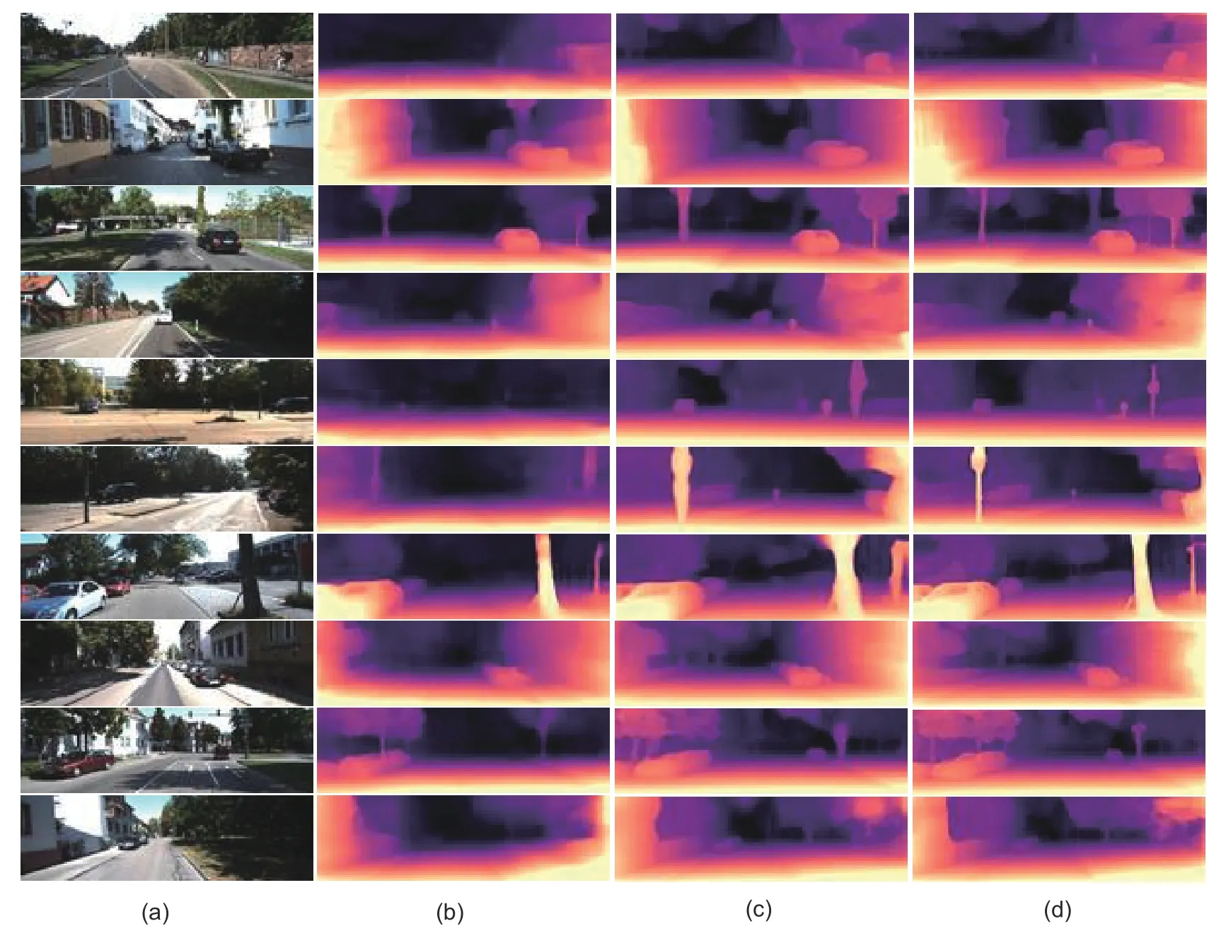
Fig.7 Qualitative comparison of our approach with state-of-the-art methods on frames from the KITTI dataset:(a) original images;(b) struct2depth;(c) monodepth2;(d) ours

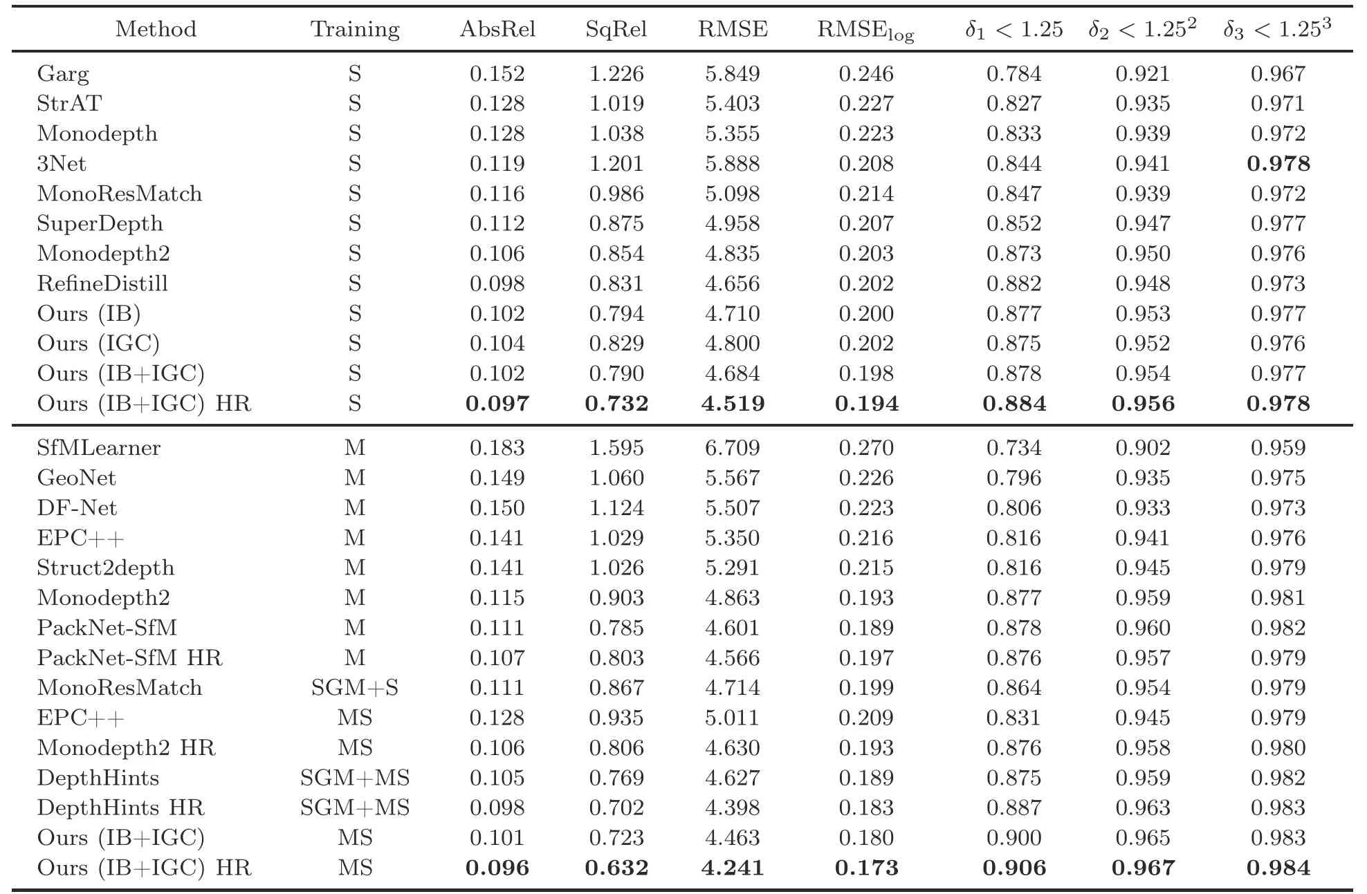
Table 1 Comparison of performances reported on the KITTI dataset

The performance metrics for depth evaluation can be defined as follows:

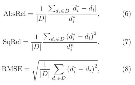
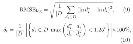
whereanddiare the ground truth and predicted depth at pixeli,respectively.Drepresents the set of all the predicted depth values of an image,and|D|is the number of elements inD.

In the quantitative experiment,DepthHints obtains a result close to that of our model.It uses a traditional stereo matching method,SGM (Gehrke et al.,2010),to provide an additional supervised signal for training,which can easily trap the optimization process in local minima.Nevertheless,the contribution values of many parameters of the algorithm that combines SGM matching and post-processing are still lower than those of our method.

4.2 Improved ground truth

The approach followed by Eigen et al.(2014),which does not deal with moving objects or obstructions,takes advantage of the re-projected LIDAR points to replace ground truth for evaluation.To further verify the effectiveness of our model,we evaluate it using the KITTI Depth Prediction Evaluation dataset (Uhrig et al.,2017),which features more accurate ground-truth depth.The new evaluation frames include 652 (or 93%) of the 697 test frames from the Eigen test split.These 652 improved ground-truth frameworks serve as a test set,and the same error metrics from the standard evaluation are used for evaluation.As shown in Table 2,our method is still significantly better than the compared methods.

4.3 KITTI ablation study

To further study the contribution of various improvements that our models provided,we carry out an ablative analysis by changing different architectural components introduced,as demonstrated in Table 3.The base architecture without any improvement has the worst effect,but when all improvements are combined,the performance is the best.

We follow a previous study(Godard et al.,2019)in initializing our models with weights pre-trained on ImageNet,because it is difficult to gain a general feature representation if training from scratch.As depicted in Fig.8b,there are obvious artifacts of in-depth maps predicted by the model lacking pre-training,and scores drop a lot in quantitative estimation.

In the Eigen split of KITTI,many low-texture areas exist in the scene,such as the car windscreen.There are almost no disparities between the two images of a stereo pair.Therefore,in the training process,pixels in this area will be re-projected to infinity.This will present a hole in the depth image,and affect the perception of an object’s structure.In Fig.8c,the parts circled in green show dilemmas such as pixel voids and incomplete shape perception caused by the absence of a mask.In addition,as shown in Table 3,the mask structure earns higher scores for the model.

Fig.8 Qualitative ablation study:(a) original images;(b) baseline;(c) no-masking;(d) ours.As the figure shows,our model with all components combined results in the finest texture and clearest outline.References to color refer to the online version of this figure

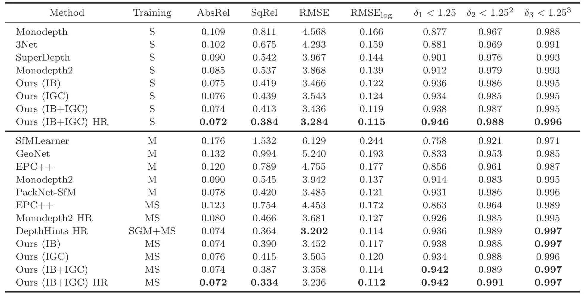
Table 2 Comparison of performances reported on the improved evaluation dataset

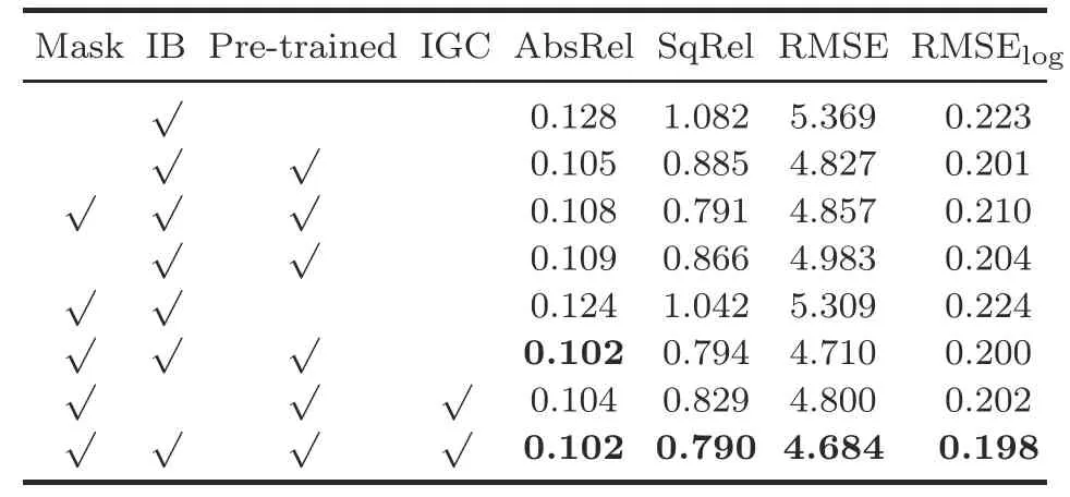
Table 3 Ablation study

4.4 Additional datasets

To illustrate the generalization performance,we extend our models to other scenes that have never appeared during training.The fashionable CityScapes(Cordts et al.,2016) and Make3D (Saxena et al.,2009)are selected as the datasets to test our monocular depth estimation models.Although there are significant differences in content,size,and camera parameters of each dataset,we still achieve a reasonable inference.

CityScapes,a semantic understanding dataset of a variety of stereoscopic video sequences recorded in street scenes from 50 different cities,contains 22 973 stereo pairs with a size of 2048×1024 resolution.However,strongly reflective Mercedes-Benz logos exist at the bottom of most images,causing the test results to deteriorate.Therefore,we use only the upper 80% of the image and discard the lower 20%.Qualitative results can be shown in Fig.9.

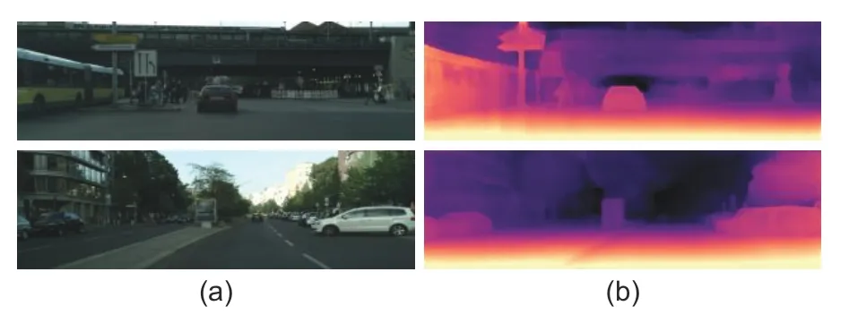
Fig.9 Qualitative results with CityScapes:(a) original images;(b) depth maps

Make3D,which has both RGB and depth maps,is used mainly for fully supervised tasks,but the number of images is small,with only 458 original pictures.Make3D (version 2) includes 458 test images.Because we used the KITTI dataset for training,its aspect ratio is quite different from that of the Make3D dataset,so we cut the randomly selected data to meet the KITTI ratio requirements.The qualitative results are shown in Fig.10.

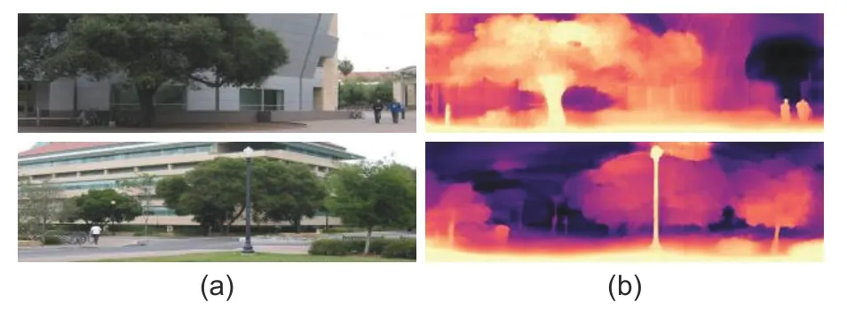
Fig.10 Qualitative results with Make3D:(a) original images;(b) depth maps

5 Discussion

In this paper,improvements are made in three aspects:backbone network,loss function,and dataset.Through an ablation study,we can see that an effective network structure and a reasonable general feature representation are the keys to improve depth estimation capabilities.

From quantitative experimental results,we can see that our model performs excellently in terms of several parameters (AbsRel,SqRel,RMSE,and RMSElog),and outperforms semi-supervised and fully supervised models,even the traditional binocular stereo vision algorithm.However,the last three parameters in Tables 1 and 2 are relatively hard to upgrade,especially the last one.We believe that this is an inherent problem with stereo input.When inputting stereo pairs for training,only the relationship between the left and right pictures is considered.When inputting sequences,the architecture will have better global characteristics,because it considers the relationship between frames.In future research,we will focus on solving the above problems,improving the effect of self-supervised depth estimation,and closing the gap between self-supervision and full supervision.

6 Conclusions

We adopted a novel monocular depth estimation backbone network,abandoning traditional ResNetbased methods.This boosted the propagation of disparate information through network layers and improved the utilization of efficient information.Furthermore,the binary mask used to deal with the pixels in the low-texture area eliminated the interference of invalid disparities in training.Finally,for more extensive and accurate general feature representation,we loaded weights that were pre-trained on ImageNet.By combining the above improvements,we produced state-of-the-art results on the Eigen split of the KITTI driving dataset using stereo pairs in a self-supervised manner(Garg et al.,2016).

Contributors

Wanpeng XU conceived and designed the method.Lingda WU and Yue QI guided the completion of the research.Wanpeng XU and Ling ZOU performed the experiments.Zhaoyang QIAN helped the experiments.Wanpeng XU drafted the paper.Lingda WU and Yue QI revised the paper.Wanpeng XU finalized the paper.

Compliance with ethics guidelines

Wanpeng XU,Ling ZOU,Lingda WU,Yue QI,and Zhaoyong QIAN declare that they have no conflict of interest.