Feature Construction and Identification of Convective Wind from Doppler Radar Data

Yuchen BAO, Juntao XUE, Di WANG, Yue YUAN, and Ping WANG

School of Electrical and Information Engineering, Tianjin University, Tianjin 300072

ABSTRACT

Key words: convective wind identification, radial velocity shear features, texture features, machine learning

1. Introduction

The convective wind is one of the common types of strong convective weather (including convective wind,hail, short-term heavy precipitation, tornadoes, etc.).Convective wind is ground-level wind with speeds greater than or equal to 17.2 m s−1that occurs due to strong atmospheric convection (Yu and Zheng, 2020). It can be local, sudden, destructive, and results in substantial economic losses every year on year. Therefore, forecasting convective wind is of great significance.

Doppler weather radar produces high spatial and temporal resolution data (Yu, 2011) and is an important data source for observing and forecasting convective wind. A variety of echo phenomena in Doppler weather radar images are associated with convective wind, such as the low-elevation severe wind area (SWA; Niu, 2014; Lagerquist et al., 2017), mid-altitude radial convergence(MARC; Schmocker et al., 1996), mesocyclones (Wapler et al., 2016), outflow boundaries, and squall lines(Klimowski et al., 2003; Yang and Sun, 2018).

The SWA refers to the region of the radial velocity image at low elevation, whose velocities are higher than a certain threshold. A low-altitude SWA often indicates catastrophic convective winds at ground level (Lagerquist et al., 2017). Niu (2014) conducted a statistical analysis of the relationship between SWA and strong convective weather and showed that SWAs are good indicators for convective wind forecasting.

MARC refers to the radial convergence zone in the mid-altitudes of a convective storm. It is known that MARC is significant when radial velocity differences of 25 m s−1or more occur in the altitudinal range of 3–7 km from the ground, and the probability of low-level winds,in this case, is significantly increased (Przybylinski,1995). Wang and Niu (2014) examined 456 samples from 30 thunderstorm and gale processes in Tianjin,China, and found that 362 of them contained significant MARCs and proposed an automatic MARC identification method. Wang and Dou (2018) improved the automatic MARC identification algorithm (Wang and Dou,2018) and detected significant MARC in 39 out of 57 strong convective processes that triggered convective winds. Yu et al. (2012) concluded that squall lines in strong vertical wind shear (WS) environments, bow echoes, supercell storms, multi-cell strong storms, and pulsating storms in weak vertical WS environments are all accompanied by MARC before producing strong surface gales. The mesocyclone is the Rankine vortex of storm-scale (1–10 km) (Wapler et al., 2016; Zhang et al.,2019). It is a critical basis for forecasting severe convective disasters, including convective winds (Wang et al.,2009).

In Doppler radar data, the SWA is a large area of high radial velocity on the radial velocity image with elevation angles of 0.5°–1.5°. MARC or mesocyclones lead to strong shear in the radial velocity image, and correspond to a strong echo cell in the reflectivity image. Therefore,high values and high shear are distinctive features of the convective wind storm region, which lays the foundation for constructing features based on radial velocity images and even reflectivity images for convective wind storm identification.

However, identifying convective wind storms based on convective wind-related echo phenomena requires accurate identification algorithms for these phenomena.Moreover, in statistical analyses of convective winds conducted by meteorologists, weakly organized storms without typical echo structures can also trigger convective winds (Yang and Sun, 2018). Therefore, more adaptable convective wind forecasting models need to be developed. Augros et al. (2013) used horizontal WS combined with four other warning rules for convective wind forecasting, thereby improving the forecasting effectiveness. Yang et al. (2018) used nine predictors for identifying convective winds and developed a forecast model using the support vector machine method. Lagerquist et al.(2017) collected U.S. radar data from 2000 to 2011 and combined them with sounding data to design and collate 431 predictors to build a convective wind forecasting model, with positive results.

The above predictive algorithms were mostly derived from predictors for identifying strong convective weather,instead of being designed for forecasting convective wind. In this respect, the present paper reports on work in which relevant features are constructed from typical radar echo phenomena of convective wind storms to establish a more adaptable model for identifying convective wind storms.

The rest of the paper is organized as follows. Section 2 introduces the data sources, data pre-processing, and calculation of labels. Section 3 introduces the methods employed, including the feature construction, principal component analysis (PCA), and the random forest model.Section 4 reports the testing and analysis, including comparing the proposed model and the severe convective wind identification model based on echo phenomena(phenomenon-based model) along with a thorough analysis of the constructed features in this paper. Section 5 summarizes the major findings of this study and suggests avenues for future work.

2. Data

2.1 Data sources and pre-processing

This paper focuses on developing a wind speed identification model with high spatial and temporal resolution using radar data. However, to understand the gap between merging and not merging environmental information into the model, versions of the model with and without the sounding data are applied in experiments to see their difference in performance. Thus, we use three types of input data, as shown in Table 1—namely, radar data, sounding data, and wind speed recording data. The radar data, obtained from the CINRAD (China New Generation Weather Radar) network deployed by the China Meteorological Administration (CMA) Public Meteorological Service Center, are used to obtain convection samples and construct features; the sounding data, from the fifth major global reanalysis produced by ECMWF(ERA5) and the NCEP Reanalysis, are used to calculate environmental parameters as features; and the wind speed recording data, from automatic meteorological stations, are used to calculate the labels of samples. We utilize these three types of data in 13 cities in China from June to August in 2016 to construct a convective wind identification dataset. The 13 cities are Tianjin, Nanjing,Shijiazhuang, Cangzhou, Yancheng, Xuzhou, Lianyungang, Changzhou, Jinan, Qingdao, Yantai, Weifang, and Binzhou.

Radar images are created by transforming the radar data from polar coordinates to Cartesian coordinates with nearest neighbor interpolation, and the resolution of an image is 1 km × 1 km in this study. The radar images include reflectivity images and radial velocity images.Each radar scans nine detection elevation angles: 0.5°,1.5°, 2.4°, 3.4°, 4.3°, 6.0°, 9.9°, 14.6°, and 19.5°. The sounding data include temperature, humidity, and wind speed data for each pressure layer and some composite variables such as convective available potential energy(CAPE) and lifting index (LI) within the radar range. The wind speed recording data comprise the maximum wind velocity per hour and its occurrence time.

Table 1. Data sources

As the ultimate aim here is to be able to provide warning for severe convective wind (SCW) by identifying severe convective storm cells, storm cell segmentation is performed to obtain the storm cells in the radar reflectivity images and filter out hyper-reflectivity via the expansion avoidance algorithm proposed by Li (2015). The reflectivity factor threshold taken for storm cell segmentation in this study is 30 dBZ. For the radar velocity data,the velocity dealiasing scheme of Yuan et al. (2020) is applied before the feature construction procedure. In order to ensure the validity of the radial velocity data, only storms located within 150 km of the radar are used as samples. For the data from automatic meteorological stations,only those records in which the wind velocity is higher than 9 m s−1are retained to calculate the labels of convective storms, as described in the following subsection.

2.2 Calculation of labels

A wind event is considered as a convective wind event if the event is observed by an automatic station in the area of a convective storm. To ensure the validity of the positive sample set and negative sample set, the rules for labeling convective wind samples are as follows:

Rule 1: If the maximum wind speed is higher than or equal to 17.2 m s−1in all wind events reported by automatic stations within the storm cell area and within 12 min of the radar scan time, the storm cell is marked as an SCW sample.

Rule 2: If a convective body satisfies Rule 1 and there is no splitting, merging, incipience, or extinction of its previous and next moment, its previous or next moment body is also marked as an SCW sample.

Rule 3: If the maximum wind speed value is within 9–15 m s−1in all wind events reported by automatic stations within the storm cell area and within 12 min of the radar scan time, and all wind events within 20 km from the boundary of the storm cell (including the area of the storm) and within 60 min of the radar scan time are less than 15 m s−1, the storm is marked as a non-strong convective wind (NSCW) sample.

According to the above rules, 13,712 convective wind samples are obtained, of which 5331 are SCW samples(positive samples) and 8381 are NSCW samples (negative samples). The sample number for each city is shown in Table 2. It should be noted that the convective wind data information identified in this paper is observed by meteorological stations, and the convective wind that does not occur at meteorological stations (such as the gale confirmed by field investigation) may not be completely recorded.

A certain number of samples can observe some echo phenomena in the sample set, such as a low-elevation SWA, MARC, mesocyclone, and squall line. The detailed statistics are shown in Table 3. If there is more than one phenomenon accompanying one convective wind sample, they are categorized in the priority order of squall line, SWA, MARC, and mesocyclone. In this paper, squall lines (Yuan and Wang, 2018), SWAs (Yuan and Wang, 2018), MARC (Wang and Dou, 2018), and mesocyclones (Hou and Wang, 2017) are obtained by intelligent identification methods.

3. Methods

3.1 Radar image feature construction

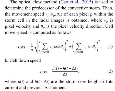
This section elaborates on the construction procedure of the radar image features used for the identification of convective wind. Five kinds of features based on the radar images are constructed by referring to the characteristics of typical convective wind-related echo phenomena, including the storm’s (1) moving speed and coresinking speed, (2) high-value reflectivity features, (3)high-value radial velocity features, (4) radial velocity shear features, and (5) radial velocity texture features.

Table 2. Sample number of each city

Table 3. Statistics of phenomena associated with convective wind in samples

3.1.1Moving speed and core sinking speed

The storm’s moving speed and core sinking speed have a directional effect on the strong convective wind(Yang et al., 2018). Zhou et al. (2011) indicated that thunderstorms move slowly during the incipient and developing phases. The mature and waning phases are influenced by fast-moving cold surface outflows, causing the storm to move fast, especially in squall lines. A straight-line wind is also usually generated at ground level when a convective core at low altitude drops rapidly in height close to the ground (Yu et al., 2006). Accordingly, two features, cell move speed (vCMS) and cell down speed (vCDS), are constructed.

a. Cell move speed

3.1.2High-value reflectivity features

The high-value reflectivity of storm cells is one of the essential features in strong convective weather forecasting. In general, the higher the value of reflectivity, the more possible it is that a convective hazard will occur.

a. Percentage of high-value reflectivity (Rref)

In the composite reflectivity (CR) image, the area of reflectivity intensity greater than or equal to 50 dBZ in the storm cells isS50, and the area greater than or equal to 40 dBZ isS40. Thus, the percentage of high-value reflectivity can be calculated as:

wherevis the point radial velocity value, andr∈{1, 2, 3}is the distance between pointspandi. The positional relationship between pointspandiis shown in Fig. 1.

A high degree of similarity is presented in the shear features because of the spatial extension of the WS field in the convective region. A mutual information (MI) calculation is introduced to reduce the number of dimensions of the similar features and retain those with higher separability.

The MI can be used to evaluate the correlation between variables (Kraskov et al., 2004) and is calculated as follows:

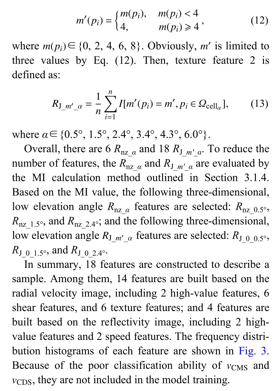
3.1.5Velocity texture features

The region of an SCW storm related to mesocyclones and MARC contains more rough texture compared to an NSCW storm. To extract the texture features of the radial velocity image of strong convective wind, the rotation invariant local binary pattern (RILBP) descriptor is chosen. The RILBP was proposed by Ojala et al. (2002)and was obtained based on the circular local binary pattern (LBP) (Ojala et al., 1994, 1996):

Calculate the number of jumpsmbetween 0 and 1 in the LBP code (LBP 0–1 and 1–0 jumps) for each point within the storm, in whichmhas five values. To set:

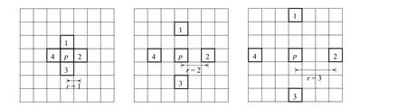
Fig. 1. The parameter r and the positional relationship between points p and i.

Fig. 2. Illustration of association points for circular LBPRq codes: (a) R = 1, q = 8; (b) R = 2, q = 16; and (c) R = 2, q = 8.

3.2 Environmental parameters

Convective parameters including CAPE, convective inhibition energy (CIN), and vertical wind shear (VWS)are generally accepted variables used in the forecasting of the likelihood and severity of an impending storm.CAPE, CIN, andKindex are extracted from ERA5; LI is extracted from the NCEP dataset; and the dewpoint, deep convective index (DCI), 700–500-hPa lapse rate (LR),and VWS are calculated from other available ERA5 products. Since there are missing values for CIN, only the MI values for the remaining seven environmental parameters are calculated. Four environmental parameters (CAPE, LI, LR, and VWS) are selected according to the MI results in Table 4.

3.3 PCA

To obtain the primary information of features, PCA is applied to the shear features and texture features. The validity and expression skill tests are performed on the combined features integrated with the principal components obtained.

PCA is a method for transforming originaln-dimensional features inton-dimensional composite features.After transformation, each principal component is a linear combination of the originaln-dimensional features and is independent of others. PCA can measure each principal component’s percentage of information. The principal component with the largest percentage of information is the first principal component, the next largest is the second principal component, and so on. In general, after transforming the original features into principal components, the feature dimension number can be compressed to just a few or even one while retaining most of the information. The higher the correlation between the original features, the smaller the number of dimensions after PCA.

3.4 Random forest model

Random forest (RF) is an ensemble-based model that uses decision trees as base classifiers. Randomly sampled subsets of training samples train each base classifier.Therefore, the trees learn in different ways, and the generalization ability of the RF model is enhanced.

This paper adopts the RF approach to construct an SCW identification model, which employs the features designed in Sections 3.1 and 3.2 as its inputs.

4. Experiments and analysis

4.1 Subsampling

The full dataset obtained as described in Section 2 is divided into a training set, a validation set, and a testing set. Storm cells on the same day are highly similar to each other. Therefore, in order to test the models properly, all samples from the same day are allocated to the same dataset. The specific partitioning is shown in Table 5.

Fig. 3. Frequency distribution histogram of each feature on SCW (red) and NSCW (blue) samples: (a) vCMS, (b) vCDS, (c) Ref99, (d) Rref, (e)Vel99, (f) Rvel, (g) shear features’ first principal component (Shearpca_1), and (h) texture features’ first principal component (VLBPpca_1).

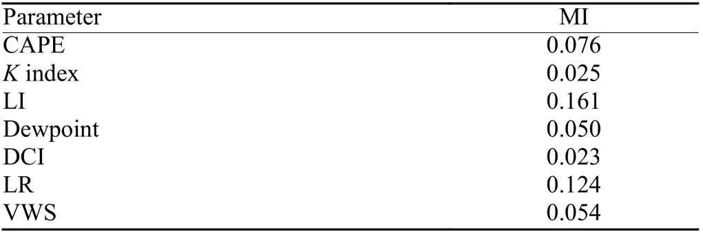
Table 4. MI values of environmental parameters

4.2 Evaluation index

In this paper, we use the probability of detection(POD), the false alarm ratio (FAR), the critical success index (CSI), and negative-case POD (NPOD) to evaluate the model, which are calculated as follows:

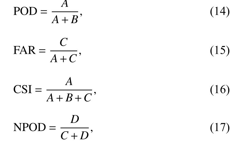
whereAis the number of SCW samples being identified as SCW,Bis the number of SCW samples being identified as NSCW,Cis the number of NSCW samples beingidentified as SCW, andDis the number of NSCW samples being identified as NSCW.

Table 5. Sample number of each sample set

4.3 Results

Experiments on the constructed datasets are carried out. Three models are trained and compared for their performance: (1) the RF model with 16 radar features constructed as described in Section 3.1, which is referred to as the radar feature model; (2) the RF model with 16 radar features and 4 environmental parameters as described in Section 3.2, which is referred to as the radar feature and EP model; and (3) the strong convective wind identification model of Lagerquist et al. (2017) as a comparison model, which is referred to as cmp-model. The cmp-model uses radar statistics, storm motion, shape parameters, and sounding indices to predict convective wind based on gradient-boosted ensembles or random forests. Except for the sounding indices, the other three kinds of predictors are utilized to construct the cmp-model in this paper to compare with the radar feature model.

All models are trained by using the training set in Table 5. Hyperparameters are chosen according to their CSI score in the validation set, and the POD, FAR, CSI,and NPOD results are recorded based on the testing set of four models. The results are shown in Table 6.

From the results, it can be seen that the performance of the radar feature model is better than that of the cmpmodel in the testing set. The POD of the radar feature model is 8.7% higher than that of the cmp-model, the FAR decreases by 1.4%, and the CSI improves by 5.9%.On the other hand, the radar feature and EP model performs better than the radar feature model, which proves that environmental parameters contribute to convective wind forecasting. However, sounding data usually have low spatial and temporal resolution, whereas the purpose here is to develop a convective wind identification model with high spatial and temporal resolution based on radar data. Therefore, the following analysis focuses on the radar features and radar feature model.

4.4 Comparative experiments with the phenomenonbased SCW identification model

Low-level SWAs, MARC, mesocyclones, squall lines,and other related phenomena are often accompanied by strong convective ground-level wind. Therefore, they are often used as a basis for judging the appearance of convective winds in practical use. Therefore, a phenomenonbased dataset is constructed with samples accompanied by SWAs, MARC, mesocyclones, and squall lines, as well as samples with no relevant phenomena. All samples in the testing set are divided into five groups: asquall line group, an SWA group, a MARC group, a mesocyclone group, and a no-relevant-phenomena group.The numbers of samples in each group are shown in Table 7.

Table 6. Comparison test results

For this section, experiments are conducted to compare the performance of the radar feature model and the phenomenon-based model on the phenomena dataset.The phenomenon-based model identifies SCW based on recognition of typical echo phenomena. If typical echo phenomena appear in radar images, the storm is judged as an SCW storm by the phenomenon-based model. It is assumed that the phenomenon-based model is ideal, i.e.,the recognition rate of the echo phenomena is 100%.Comparisons with this idealized model can reveal the performance quality of the developed model when the convective wind is not caused by the relevant phenomena. Each group is tested separately by using the radar feature model, and the test results are shown in Table 8.

From the results in Table 8, it is apparent that:

(1) For the phenomenon-based model, the POD for each phenomenon group and the NPOD for the no-relevant-phenomena group are 100%. This is inevitable under the assumption that the recognition algorithm is perfectly correct. The NPOD for each phenomenon group and the POD for the no-relevant-phenomena group are zero. This is because the phenomenon-based model does not have the ability to identify SCW samples without phenomena, and will identify all NSCW samples with phenomena as SCW, which are its major drawbacks.

(2) For the radar feature model, the POD and FAR for each phenomenon group are better than those for the norelevant-phenomena group. The reason is that the features of the radar feature model are constructed according to the characteristics of typical phenomena related to convective wind. Meanwhile, there is a higher NPOD forthe no-relevant-phenomena group.

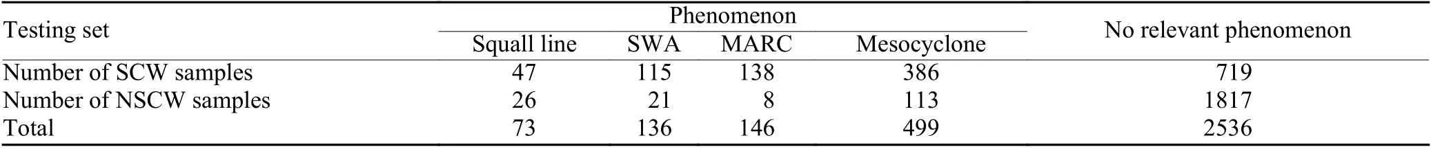
Table 7. Numbers of samples in each phenomenon group

Table 8. Test results of the radar feature model and phenomenon-based model

(3) For each phenomenon group, the POD of the phenomenon-based model is better than that of the radar feature model. However, the FAR of the radar feature model is lower than that of the phenomenon-based model, resulting in a higher CSI. This makes sense because the radar feature model has some ability to identify NSCW samples with phenomena.

(4) For the no-relevant-phenomena group, the POD of the radar feature model increases by 66.8% compared to the phenomenon-based model, accompanied by a decrease in NPOD of approximately 14.6%. This proves that the radar feature model is more advantageous than the phenomenon-based model for identifying no-relevant-phenomena SCW samples.

(5) For all samples in the phenomenon dataset, with a sample ratio of 1245 : 1992, higher POD, FAR, and CSI values are delivered by the radar feature model, accompanied by a certain decrease in NPOD, which is acceptable. It can be concluded that the model developed here has a strong ability to identify SCW samples with phenomena, whilst at the same time having some ability to discriminate between SCW and NSCW samples without phenomena.

4.5 Feature testing and analysis

Two experiments with all samples in Table 3 are conducted in this part of the study to test the validity of the speed features, high-value reflectivity and velocity features, shear features, and texture features: experiment 1 is designed to test the performance of SCW samples and NSCW samples, and experiment 2 to test the performance of SCW samples with and without phenomena.

4.5.1Feature pre-processing

a. PCA results of shear features

The shear features obtained according to the method described in Section 3.1.4 have 54 dimensions. Furthermore, the interdependency among the shear features creates a high degree of information redundancy. Therefore,PCA is applied as described in Section 3.3 to transform the 54-dimensional features and reduce the dimensionality. The information percentage of each principal component is obtained, as shown in Table 9. It can be seen that the information content of the first principal component is 86.3%. Therefore, the shear features’ first principal component Shearpca_1is chosen to represent the 54-dimensional original shear features for the feature validity analysis.

b. PCA results of texture features

The texture features obtained according to the method described in Section 3.1.5 have 18 dimensions. The PCA method is again applied, and each principal component’s information percentage is obtained, as shown in Table 10. The information of the first principal component accounts for more than 60%, so the first principal component VLBPpca_1of the texture features is chosen to represent the 18-dimensional original texture features for the feature validity analysis, as follows.

4.5.2Performance of features in SCW and NSCW identification

The classification capabilities of the different features includingvCMS,vCDS, Ref99,Rref, Vel99,Rvel, Shearpca_1,and VLBPpca_1need to be analyzed. To this end, the frequency distribution histogram of each feature is shown in Fig. 3.

As can be seen from the distributions shown in Fig. 3,in terms of the separability of strong convective wind samples from non-strong convective wind samples:

(1) The best performance appears with Shearpca_1and VLBPpca_1. Specifically, it can be stated that the variability of the shear and texture features based on radial velocity images is greater in these two sample sets. This is because storms that generate convective winds are usually accompanied by strong atmospheric motion, resulting in more shear in the radial velocity images.

(2) The Vel99andRveldirectly reflect the speed and high-value ratio of particle motion within the storm. The Ref99andRrefdirectly reflect the storm intensity. Their performances are acceptable. As intensity increases, the possibility of convective gales will increase.

(3) The histogram distributions ofvCMSandvCDSare almost indistinguishable, indicating that for convective wind storms, these two features have little ability to classify SCW samples and NSCW samples.

4.5.3Performance of features in classifying SCW sample sets with echo phenomena

To evaluate the performance of features in classifying SCW samples with SWAs, MARC, mesocyclones, and squall lines, histogram statistics are calculated and compared with the feature distributions of SCW samples without these phenomena.

a. Performance of radial velocity high-value features in

SCW samples with SWAs

Table 3 shows that, among the 689 convective wind samples with SWAs, SCW is observed in 556 samples,accounting for 80.7%. To verify the descriptive ability of the feature to the SWA, the high-value featuresRveland Vel99of the radial velocity associated with SWAs are chosen. The distribution of features is shown in Fig. 4,using 4775 samples of SCW samples without SWAs and 556 samples of SCW samples with SWAs, as in Table 3.

Table 9. Information percentages of shear features

Table 10. Information percentages of texture features

Radial velocity high-value features for SCW samples with SWAs have overall higher values than those without SWAs. This indicates that these two features, which already have ability to distinguish between SCW and NSCW samples, will have even more ability to distinguish between SCW samples with accompanying SWAs.

b. Performance of shear and texture features in SCW sample sets with MARC and mesocyclones

From the samples collected in Table 3, it can be seen that, among the 516 samples of convective wind with significant MARC, there are as many as 493 SCW samples, accounting for 95.5%; plus, among the 1962 samples of convective wind samples with mesocyclones,there are 1592 samples reaching the strong convective wind level, accounting for 81.1%. Both MARC and mesocyclones are associated with stronger atmospheric motions such as convergence, dispersion, and rotation.Therefore, the shear feature Shearpca_1and texture feature VLBPpca_1are chosen. Figure 5 shows the feature distributions of 4838 samples of SCW without MARC and 493 samples of SCW with MARC. Figure 6 shows the feature distributions of 3739 samples of SCW without mesocyclones and 1592 samples of SCW with mesocyclones, as in Table 3.

From the results, it can be seen that: (1) the ranges of the texture feature value domain of the SCW sample set containing MARC or mesocyclones are overall higher than those of the SCW sample set without MARC or mesocyclones; (2) combined with Figs. 3g, h, the indication is that, for SCW samples containing MARC or mesocyclones, they can be further distinguished from NSCW samples in terms of shear and texture features.

c. Performance of moving speed features in SCW samples presenting squall lines

Squall lines are usually accompanied by thunderstorms, high winds (or tornadoes), and hail, and are characterized by high energy and destructive power. As shown in Table 3, a total of 286 samples of squall line samples are included in the dataset, among which 206 samples of SCW occur, accounting for 72.0%. Considering the separate tests and discussions carried out for the possible low-level SWAs, MARC, and mesocyclones in a squall line, as well as the high-moving-speed characteristics of squall lines, the focus here is only on the tests of the single-body moving speed featurevCMS, and the distribution of this feature organized with the samples in Table 3 is shown in Fig. 7.

Looking back at Fig. 3a, thevCMSis not very skilled at distinguishing between SCW and NSCW samples, while Fig. 7 demonstrates that SCW caused by a squall line tends to show a strongervCMS, thus illustrating the usefulness of the “storm moving speed” feature.

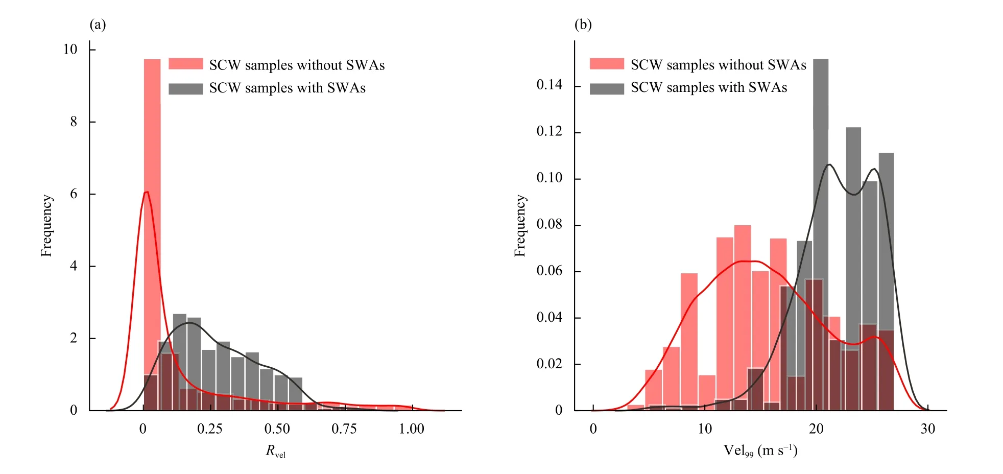
Fig. 4. Frequency distribution histograms of radial velocity high-value features in the sample set of SCW samples with SWAs (black) and without SWAs (red): (a) Rvel and (b) Vel99.

Fig. 5. Performance of (a) Shearpca_1 and (b) VLBPpca_1 in classifying SCW samples with/without MARC.

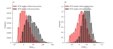
Fig. 6. Performance of (a) Shearpca_1 and (b) VLBPpca_1 on SCW samples with/without mesocyclones.

In summary, except for the weak ability of the moving speed features, all the other three kinds of features(i.e., high-value, shear, and texture features) constructed in this study perform well in identifying SCW and NSCW. Also, the value of SCW samples accompanied by the phenomena of SWAs, MARC, and mesocyclones,is always higher than without these phenomena. Moreover, the model has some ability to express SCW samples that do not show these phenomena.

4.6 Typical examples

In the test sample set, three cases of convective winds with continuous scans are selected to highlight the model’s ability to identify convective storms in advance and to compare the main features used. The first two cases are convective storms with and without the typical echo phenomenon (MARC), and the third case is a convective storm whose wind does not reach the level of strong convective winds. The detection radar, time, and number of body scans are shown in Table 11. Figure 8 presents their detailed timing information, including the maximum wind speed under the relevant single body (within 6 min after the volume scan time) for each case of the body-bybody scan, the occurrence of typical echo phenomena,and the model’s body-by-body scan prediction results.

As shown in Fig. 8, the model correctly identifies convective storms with or without MARC, and identifies them six body scans (Case 1) earlier than the appearance of MARC and four body scans (Case 2) earlier than the appearance of strong winds on the ground. Also, the model correctly identifies Case 3 as NSCW at all times.

In order to illustrate the performance of the extracted features in different types of convective wind sequences intuitively, two single reflectivity high-value features(2/2), two radial velocity shear features (2/6), one radial velocity texture feature (1/6), and one radial velocity high-value feature (1/2) are selected in four categories of 16-dimensional features to form three two-dimensional feature diagrams and conduct a comparative analysis.

First, the reasons for selecting the six features mentioned above are as follows:

(1) Compared with the number of radial velocity features, fewer features are based on single reflectivity. All the high-value reflectivity features,Rrefand Ref99, are selected and made to form a two-dimensional feature diagram (Fig. 9a).

Fig. 7. Performance of the moving speed feature in SCW sample sets with/without squall lines.

(2) For the high-value radial velocity, shear, and texture features, two two-dimensional feature diagrams are formed: “high-value radial velocity and shear” (Fig. 9b)and “shear and texture” (Fig. 9c). In the “high-value and shear” diagram, the high-value feature uses Vel99and the shear feature usesRWS_3_6_4.3°. In the “shear and texture”diagram, the texture feature usesRJ_0_0.5°and the shear feature usesRWS_3_4_0.5°, which is at the same elevation angle.

Scatter diagrams for the three cases are shown in Fig.9, from which it can be seen that:

(1) All four types of features show very high discrimination between SCW and NSCW in all three cases.

(2) For the high-value reflectivity features (Fig. 9a),the ability to distinguish the presence or absence of typical echo phenomena mainly results from the Ref99feature.

(3) For both the high-value radial velocity feature and the radial velocity shear feature (Fig. 9b), convective storms accompanied by MARC are stronger than those without typical echoes. At the same time, these two types of features do not show a strong correlation for convective storms without typical echoes.

(4) The nonlinear distribution of the case sample in the“shear and texture” feature plane presented in Fig. 9c indicates that these two types of features are not highly correlated, and their roles in the model cannot be replaced by each other.

5. Summary

Fig. 8. Detailed timing information for three cases, including the maximum wind speed under each individual body scan, the occurrence of typical echo phenomena, and the model’s prediction results.

The objective of this study is feature construction for severe convective wind and building of a model to identify the SCW. To this end, a single storm cell with a maximum ground wind speed of more than 17.2 m s−1is regarded as an SCW sample, while wind speeds within 9–15 m s−1are considered to be NSCW samples.

A dataset is constructed by using the radar images and data from automatic meteorological stations in 13 cities of China from June to August 2016. Five kinds of features are constructed by referring to the characteristics of typical convective wind-related echo phenomena, and a model for identifying SCW is built.

Results from testing the model and validity of the features indicate that most features perform well in distinguishing SCW and NSCW, and excel at distinguishing SCW from NSCW when carrying typical phenomena.

At the same time, according to the radar feature and EP model results in Table 6, environmental parameters have a positive effect on the identification of convective wind. However, sounding data usually have a low temporal resolution (recorded at 0800 and 2000 BT) for realtime forecasting. Therefore, it is not easy to guarantee the validity of sounding data in practical use. It would be worthwhile exploring how to effectively use the information provided by environmental physical fields to jointly train a stronger convective wind recognition model with higher quality, which is the next step for our group in future work.

Acknowledgments.The authors thank the CMA Public Meteorological Service Center for providing the source data.