Some Research on Limit Cycles of Liénard System
2021-11-08 13:49:12YangRuochengYangLiuqingTangYilei
数学理论与应用 2021年3期
Yang Ruocheng Yang Liuqing Tang Yilei
(1.School of Mathematical Sciences,Shanghai Jiao Tong University,Shanghai 200240,China;2.College of Mathematics and Computer Science,Fuzhou University,Fuzhou 350108,China)
Abstract The aim of this paper is to introduce the progress on the research for limit cycles of Liénard systems and present some new results.The results focus on four problems:the existence,the uniqueness,the exact number and the upper bound of limit cycles.We also summarize some methods for studying the limit cycles of Liénard systems.
Key words Limit cycle Liénard system Existence and uniqueness of limit cycles Exact number of limit cycles
1 Introduction
Hilbert’s 16th problem was proposed by Hilbert at the International Congress of Mathematicians in 1900,as one of the 23 problems in mathematics.The second part of the problem is related to the upper bound for the number of limit cycles in plane polynomial vector fields of degreenand their relative positions,which remains open forn>1.
In 1923 Dulac[1]tried to prove that each given polynomial system has a finite number of limit cycles but a serious leak of his proof was found about 60 years later,Yu.Ilyashenko[2]and Ecalle[3]patched up in two long articles.See more details of results of Hilbert’s 16th problem in[4–8].
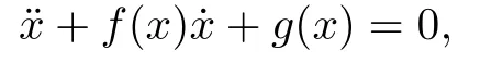
Smale listed Hilbert’s 16th Problem as one of the most elusive mathematical problems(see Question 13 in [9]),and said:“Except for the Riemann hypothesis it seems to be the most elusive of Hilbert’s problems.”Therefore,Smale [10] suggested to study Hilbert’s 16th problem restricting on the Liénard system[11],which is a second order differential equation,named after the French physicist and engineer Alfred-Marie Liénard.Letfandgbe two continuously differentiable functions on R.Consider the Liénard equation

wherex ∈R and functionsf,gsatisfy the conditions for the existence and uniqueness of solutions with respect to initial values.In application−g(x)usually represents the restoring force of a spring andrepresents the frictional force.
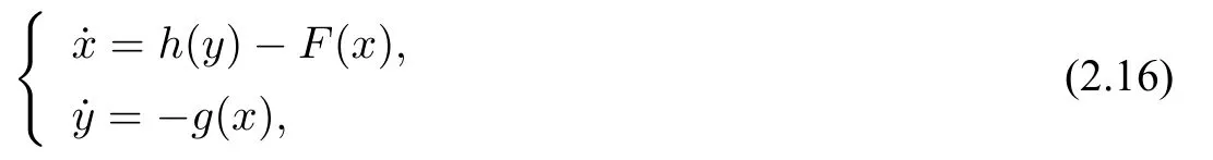
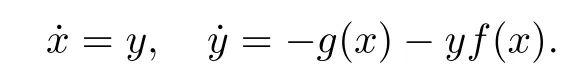
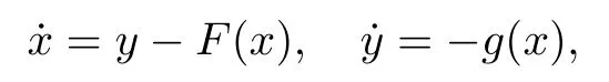
The equation(A1)can be transformed into two equivalent two-dimensional systems,
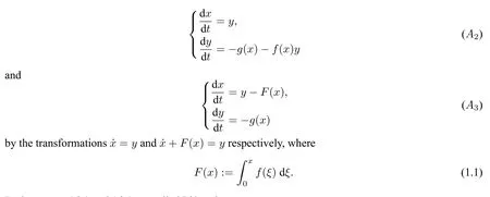
Both systems(A2)and(A3)are called Liénard systems.
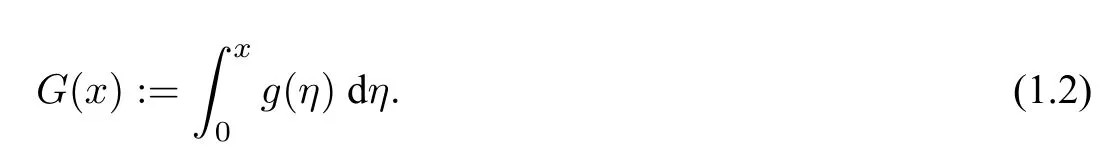
Let
In view of the Hilbert’s 16th problem,we are mainly concerned with the theory of existence,stability,hyperbolicity,number of limit cycles and their relative positions on the study of limit cycles of Liénard systems.The organization of this paper is as follows.In section 2,we introduce the results on the study of limit cycles of Liénard systems,concerning the following four problems:
Problem(A)Does a limit cycle exist for a Liénard system?
Problem(B)Is the limit cycle unique for a Liénard system?
Problem(C)What is the exact number of limit cycles for a Liénard system?
Problem(D)What is the upper bound of limit cycles for a Liénard system?
Section 3 is devoted to the brief introduction of the methods for studying the Liénard systems.
2 Limt cycles of Liénard systems
In this section,we summarize the results on the study of limit cycles of the Liénard systems(A1)–(A3)focusing on the four problems(A)–(D)in Introduction.Moreover,we sort out the results with respect to smooth or piecewise smooth systems in subsections.
2.1 Existence of limit cycles
2.1.1 Smooth systems
The following results has mainly referred to the works [12] and references therein.Consider the classical Liénard differential equation of form(A1)

whereg(x)∈C1.Lety=dx/dt,then

whereG(x)is defined by(1.2)andCis an arbitrary constant in R.(2.4)provides a first integral of(2.3).Note thatm y2/2 represents the kinetic energy andm G(x)represents the potential energy,wheremis the mass.This equation may have periodic solutions but cannot exist limit cycles.It is not difficult to obtain the global dynamics of this equation.
In 1926,in order to study the constant amplitude oscillations of a triode vaccum tube,Van de Pol considered the equation(A1)with
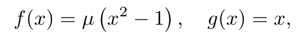
i.e.,the Van de Pol equation,and proved the existence of an isolated closed orbit,where parameterµ∈R+.In 1928,Androv combined the work of Van de Pol with the theory of Poincaré on limit cycles to obtain a series of results.
Theorem 2.1([13]) Suppose that
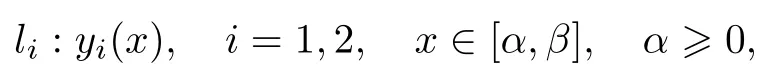
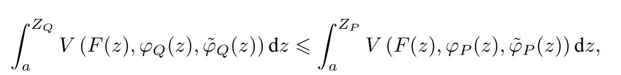
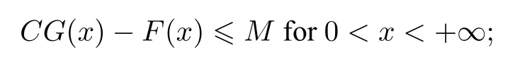
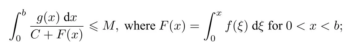
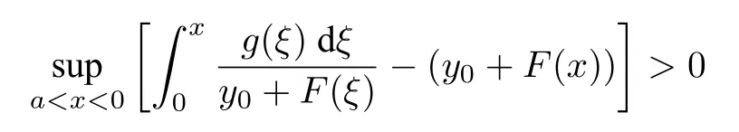
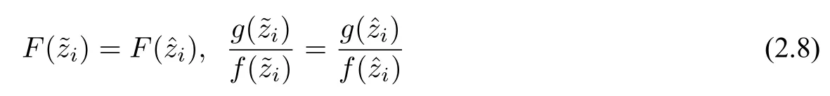
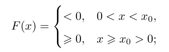
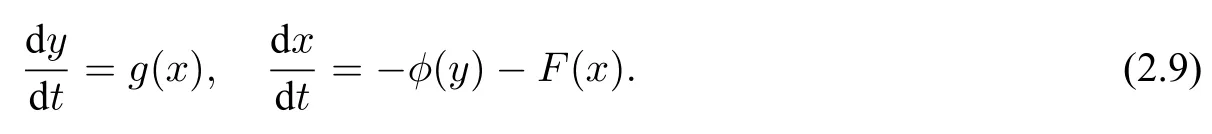
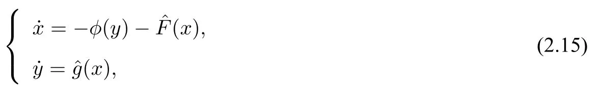
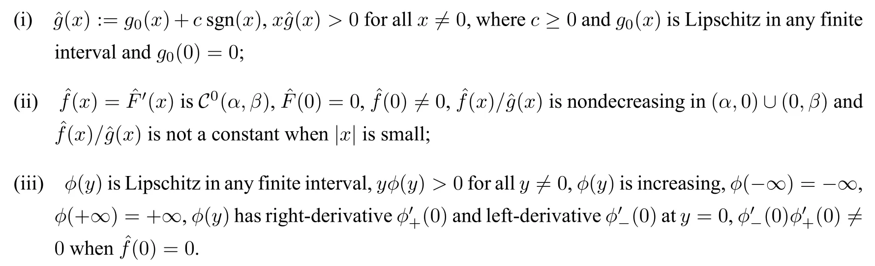
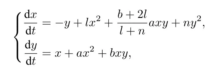
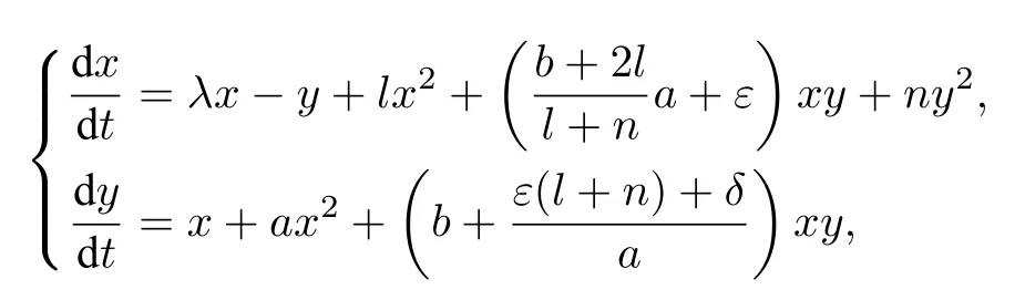
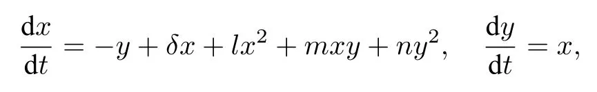
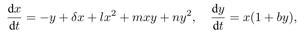
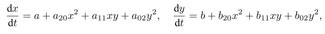
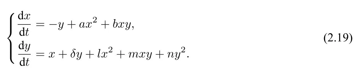
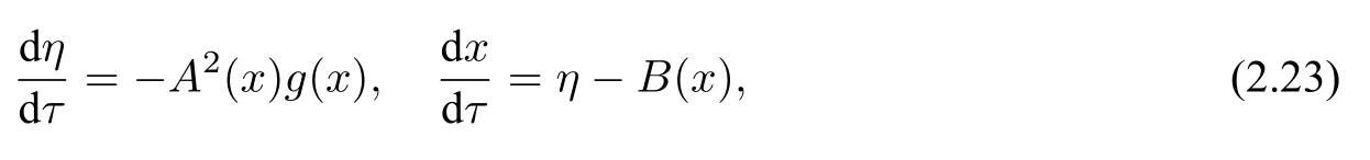
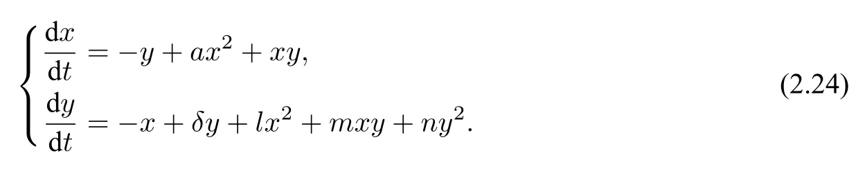
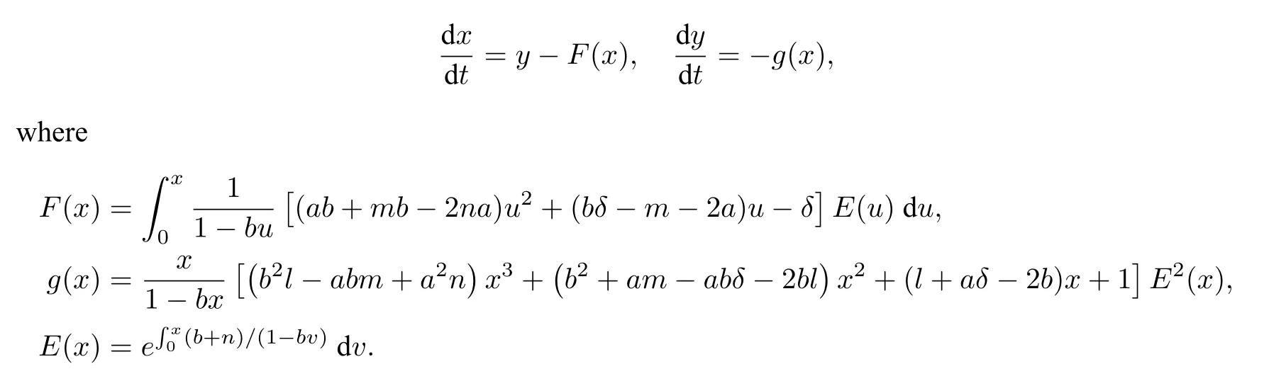
(1)F(x) andg(x) satisfy the Lipschitz condition for|x| (2)xg(x)>0 forx0,andG(±∞)=+∞,whereG(x)is shown in(1.2); (3)F(x)<0 for 0 (4) there exist a constantM >max(x1,|x2|)and two numbersk1,k2satisfyingk2 Then system(A3)has at least one closed orbit. In addition,Huang[14]first improved Dragilev’s theorem by weakening hypothesis(4)in Theorem 2.1.Later,Ding [15] extended the results further by replacing the hypothesis (4) with the following condition: (5)There exist a constantM >max(x1,|x2|)and a numberksuch thatF(x) ≥kforx≥MandF(x)≤kforx≤−M.Moreover,either In[16],Gao and Ding also extended the above existence theorem to a generalized Liénard equation. Furthermore,by using Filippov’s transformation with its inverse transformationx=xj(z)and letting forj=1,2,system(A3)can be converted to the equivalent system Theorem 2.2([17],Fillipov’s theorem) Suppose that (1)f(x),g(x)are continuous,xg(x)>0 forx0,andG(±∞)=+∞; (2) there exists a parameterδ >0 such that if 0 (3) there exists az0>δ,such that>0,and whenz >z0,F1(z) ≥F2(z), Then system(A3)has at least one closed orbit. Hypothesis(1)in Theorem 2.2 is generally necessary which can insure that the system has a unique critical point.Obviously,with the aid of Fillipov’s theorem,there exist examples with at leastnlimit cycles by changing the signs ofF1(z)−F2(z). Theorem 2.3([18]) Suppose that (1)xg(x)>0 forx0,G(−∞)=+∞,xF(x)<0 for 0<|x|<δ; (2) there exist two positive constantsCandMsuch that (3) there exist two positive constantsx0andksuch thatf(x)/g(x) ≤kforx <−x0,andM+1/C+F(−x0)≤1/k; Then system(A3)has a closed orbit. In the above three theorems we see thatxg(x)>0 forx0 is always required in order to make the positive semiorbit of system(A3)to spiral around the origin.Moreover,some of the following conditions are usually needed: In [19],Zhou found several sufficient conditions for the existence of closed orbits when at least two of the above conditions are invalid.Later,Ding [15] obtained a series of new sufficient conditions for the existence of closed orbits of system(A3). The following theorem removes the conditions in (2.7) and gives the region where the limit cycle exists. Theorem 2.4(Zhang[12]Chapter 4) Suppose that (1)g(x),f(x)∈C0,xg(x)>0 forx0,a (2) there exist two positive constantsCandMsuch thatC+F(x)>0,and (3) if infa holds; (4) one of the following is true: (a)G(b)≥(y0+y1)2/8, (b) sup0 whereG(x)=supa Then system(A3)has a closed orbit in the generalized rectanglea Chen and Tang in[20]considered the Liénard system(A3)and gave the non-existence of closed orbits withFandgof classC(R)in(β1,β2),whereβ1<0,β2>0 andβ1,β2can be∓∞. Theorem 2.5([20]) WhenF(x)andg(x)in system(A3)satisfy the following conditions(i)-(iv): (i)xg(x)>0 forx ∈(β1,0)∪(0,β2); (ii)F(x)has at most three zerosx1,x2,0∈(β1,β2)withx1 (iii)f(x)=F′(x)has a unique zeroξ0in(x1,x2),andf(x)<0(resp.>0)forx ∈(ξ0,x2)(resp.x ∈(x1,ξ0)∪(0,β2)); (iv) the simultaneous equationsF(z1)=F(z2) andhave no solutions in (β1,β2)satisfyingx1 Theorem 2.6([20]) WhenF(x)andg(x)in system(A3)satisfy the following conditions(i)-(iv): (i)xg(x)>0 forx ∈(β1,0)∪(0,β2); (ii)F(x)has two zeros0∈(β1,β2)with≤0; (iii)f(x)=F′(x)has a unique zeroandf(x)<0(resp.>0)forx ∈(resp.x ∈ (iv) whenF(z1)=F(z2)forz1,z2∈1≤i ≤n,the inequality asz1<<0 hold, then system(A3)has no closed orbits. 2.1.2 Non-smooth systems Differential equations derived from practical problems often have of non-smooth properties,such as derivative discontinuity or discontinuous jump points.Therefore,the research of such systems has attracted much attention. In 2020,Chen and Tang[21]gave the following theorem for the existence and uniqueness of closed orbits for a piecewise smooth Liénard system. Theorem 2.7Consider the Liénard system(A3)and assume the following conditions: (1)g(x)is an odd function andxg(x)>0 forx ∈(−∞,0)∪(0,+∞); (2)F(x)is an odd function,F(x0)=0 for somex0>0 and (3) (4)F(x)is Lipschitz continuous in any bounded interval and increase forx >x0,andg(x)is Lipschitz continuous forx ∈(−∞,+∞){0,±x1,...,±xn}. Then,system(A3)has a unique limit cycle,which is stable. 2.2.1 Smooth systems Concerning the uniqueness of limit cycles,there are many important results for the Liénard’s equations.We introduce part of them which are related to our research. Theorem 2.8([22]) Suppose that the following conditions are satisfied: (1)g(x)is an odd function,andxg(x)>0 forx0; (2)F(x)is an odd function,and there exists anx0>0 such thatF(x)<0 for 0 (4)f(x)andg(x)satisfy the Lipschitz condition in any bounded interval. Then system(A3)has a unique limit cycle which is stable. Sansone [23] put forward the following results which can deduce Theorem 2.8.Meanwhile,by weakening the condition of Theorem 2.9,Sansone obtained the same conclusion in Theorem 2.10. Theorem 2.9([23]) For system(A3),assumeg(x)=x.Suppose that the following conditions are satisfied: (1)f(x)∈C0(−∞,∞),and there exist two parametersδ−1<0<δ1such thatf(x)<0 forδ−1 (2) there exists a constant ∆>0 such thatF(∆)=F(−∆)=0; (3)F(+∞)=+∞,orF(−∞)=−∞. Then system(A3)has a unique limit cycle which is stable. Theorem 2.10([24]) Suppose thatg(x)=xandf(x)satisfies the following conditions: (1)f(x)∈C0(−∞,+∞),f(x)<0 for|x|<δandf(x)>0 for|x|>δ >0; (2)F(+∞)=+∞,orF(−∞)=−∞. Then system(A3)has a unique limit cycle which is stable. By using the fact that all closed orbits are of star-type,Massera[25]obtained the following results. Theorem 2.11([25]) Consider system (A3) and letg(x)=x.Suppose thatf(x) satisfies the following conditions: (1)f(x)∈C0(−∞,+∞); (2) there exist two parametersδ−1,δ1such thatf(x)<0 forδ−1 (3)f(x)is nondecreasing as|x|increases. Then system(A3)has a unique limit cycle which is stable. Zhang[26]improved the results by replacing hypothesis(3)in Theorem 2.11 with hypothesis(2)in Theorem 2.12. Theorem 2.12([26]) Suppose that the following conditions hold: (1)xg(x)>0 forx0,G(x)=∫satisfiesG(±∞)=+∞,g(x)is continuous and satisfies the Lipschitz condition in any finite interval; (2)f(x)is continuous,andF(x(u))/uis nondecreasing in|u|,whereF(x)=andx=x(u)is the inverse function ofu=u(x)= Then system(A3)has at most one limit cycle. Suppose thatf(x) has two zerosx1,x2withx1<0,x2>0.What additional conditions do we have to give to ensure that the Lienard equation has a unique limit cycle? To answer this question,Zhang presented the following Theorem[26,27]. Theorem 2.13([26]) Consider system(A3)and letg(x)=x.Suppose thatf(x)∈C0(−∞,+∞),f(0)=0 andf(x)/xis nondecreasing forx ∈(−∞,0)∪(0,∞).Then system(A3)has at most one limit cycle.It is stable if it exists. Meanwhile,Zhang gave the following result by applying the transformationu= Theorem 2.14([26]) Suppose that the following conditions hold: (1)xg(x)>0 forx0,G(−∞)=G(+∞)=+∞whereG(x)=andg(x)is continuous and satisfies the Lipschitz condition in any bounded interval; (2)f(x) is continuous,andf(x)/g(x) is nondecreasing inx,forx ∈(−∞,0)∪(0,+∞); andf(x)/g(x)0 in a neighborhood ofx=0. Then system(A3)has at most one limit cycle,and the limit cycle is stable,if it exists. In[28],Cao and Liu considered the symmetric Liénard system and developed a method to give the bound of the amplitude of the unique limit cycle.As an application,they also considered the van der Pol equation=y −µ(x3/3−x),=−x,whereµ>0. The following theorem is proved in[26]and[27]for generalized Liénard systems. Theorem 2.15([27]) Consider the system Suppose that in addition to the hypothesis in Theorem 2.14,the following conditions are satisfied:yϕ(y)>0 fory0;ϕ(±∞)=∞;ϕ(y) is continuous,monotone,and satisfies the Lipschitz condition; the functionϕ(y)has left and right derivativesaty=0 with0.Iff(0)=0,then the system can have at most one limit cycle,and the limit cycle is stable,if it exists. Assume that there existx2<0 Theorem 2.16([29]) Consider system(2.9)forF(x)=Suppose that for everyx ∈(a,b)with−∞≤a<0 (1)xg(x)>0 forx0 andyϕ(y)>0 fory0; (2)f(x),g(x),ϕ(y)are continuously differentiable,ϕ(y)is monotonically increasing andf(0)<0(orf(0)>0); (3) there exist two constantsα,βsuch thatf1(x)=f(x)+g(x)[α+βF(x)]has simple zerosx1<0 andx2>0,andf1(x)≤0(orf1(x)≥0)in the interval(x1,x2); (4) the functionf1(x)/g(x)is nondecreasing(or nonincreasing)outside the interval[x1,x2]; (5) each closed orbit encloses the interval[x1,x2]on thex-axis. Then system(2.9)has at most one limit cycle,and the limit cycle is stable(or unstable)if it exists. Theorem 2.17([30]) Consider the generalized Liénard system whereF,g,h ∈C(R),and assume that system(2.10)satisfies the following conditions: (1) there is a positive numbera1such thatFdoes not change sign on[0,a1]and is not identically zero withF(0)=F(a1)=0; (2)g(x)>0 forx>0; (3)his strictly increasing and odd,i.e.,h(−x)=−h(x)for allx ∈R; (4)h(R)⊃F(R); (5)ϕ:I →Jis weakly increasing,absolutely continuous,and≥g(x)for a.e.x ∈I; (6) for the functionϕsatisfying (5) we have sgnF(ϕ(x))=−sgnF(x),sgnF(−ϕ(x))=−sgnF(−x),|F(ϕ(x))|≥|F(x)|,and|F(−ϕ(x))|≥|F(−x)|for allx ∈I. Let 0=a0 In the following,we will present two uniqueness theorems[31].They include some usual uniqueness results concerning system (A3) as particular examples.The corollary of Theorem 2.18 introduces a“determining”functionF(x)/Gα(x),α≥0.The functions of Theorem 2.8,Theorem 2.9,Theorem 2.11,and Theorems 2.12,2.13,2.14 can be considered as special cases corresponding toα=0,1/2,and 1,respectively.Moreover,Theorem 2.10 is naturally a special case of Theorem 2.18.Consequently,the unique limit cycle in the above theorems is simple. Suppose that(A3)is defined in the stripx02 Denotez0i=G(x0i),i=1,2,z0=min(z01,z02).Letxi(z) represent the inverse function ofz=G(x)for(−1)i+1x≥0,respectively fori=1,2.By Filippov’s transformationx=xi(z),i=1,2,system(A3)can be respectively written in the regionsx≥0 andx≤0 as(E1)and(E2),where andFi(z)=F(xi(z)). Theorem 2.18([31]) Suppose thatf(x),g(x) are continuous in (x02,x01) andxg(x)>0 forx0.Assume that (1) there exists ana,0 ≤a≤z0such thatF1(z) ≤0 ≤F2(z)for 0 (2)≤0 for 0 (3) for any constantk≥1,ifHk(z)=F2(u) foru≥z≥a,thenwhereHk(z) is defined as Then in the stripx02 Theorem 2.19([31]) Suppose thatf(x),g(x)are continuous in(x02,x01),xg(x)>0 forx0,and the following conditions are satisfied: (1) there exists ana ∈[0,z0)such thatF1(z)≤0 ≤F2(z)for 0 (2)≤0 ifF2(z)<0 for 0 (3)is nondecreasing forz >is nondecreasing forz >0 andF1(z01−0)≤F2(z02−0)); (4)ifF1(z)=F2(u)foru≥z >a. Then there exists at most one limit cycle for(A3)inx02 Definea∗≥0 by the relationa=G(a∗),then the following conditions(3*),(4*)are respectively equivalent to conditions(3),(4)in Theorem 2.19. (3∗)F(x)f(x)/g(x) is nondecreasing in (a∗,x01) (or nonincreasing in (x02,0) andF(x01−0) ≤F(x02+0)). (4∗) For any constantc >0,the two curvesF(u)=F(x)andG(u)=G(x)+ccan intersect at most one point in the regiona∗≤x Considering the possibility to generalize Massera’s uniqueness theorem (Theorem 2.11) to the equation=0,we present the conjecture of De Castro[32]. Conjecture 2.1Consider the differential equation or its equivalent system Assume that: (1)g(x)is continuous and satisfies the Lipschitz condition,xg(x)>0 forx0,G(+∞)=+∞whereG(x)=andg(x)is nondecreasing asxincreases; (2)f(x,v) is continuous and satisfies the Lipschitz condition with respect toxandv,f(0,0)<0 andf(x,v)>0 for|x|>a>0; (3) there exist two constantsN >0 andα>0 such that any continuous functionv(s)satisfying|v(s)|>Nmust have the property≥α>0 for|x|>a; (4)f(x,v)is nondecreasing as|x|and|v|increase. Then system(2.14)has a unique limit cycle. The uniqueness part of the conjecture 2.1 forg(x)=xholds if the”nondecreasing”in hypothesis(4)is substitued by”strictly increasing”([12,Chapter 14]). In 2015,Yang proved that the Liénard system (A3) with symmetry (i.e.,F(x) andg(x) are odd functions) has a unique limit cycle under some hypotheses.The unique limit cycle locates in the strip region|x| Theorem 2.20([33]) Consider system (A3) withg ∈C(R) andF ∈C2(R),which satisfies the following conditions: (i)xg(x)>0 forx0,x ∈(β1,β2); (ii)F(0)=0; (iii)f(x)=F′(x)has a unique zero 0 andf(x)<0(or>0)asβ1 (iv) the equations(2.8)has at most one solution Moreover,whenF(x1)=F(x2),λ(x1)>λ(x2)(resp.F(x1)=F(x2),λ(x1)<λ(x2))as|x1|,|x2|are small,system(A3)satisfies either(v)or(v′),where:=g(x)/F(x): (v) the functionF(x)f(x)/g(x)is decreasing(resp.increasing)forβ1 (v′) the functionF(x)f(x)/g(x)is increasing(resp.decreasing)for 0 Then system(A3)has at most one closed orbit in the region{(x,y)∈R2:β1 2.2.2 Non-smooth systems Based on the uniqueness theorem of Zhang in [27] on the number of limit cycles of the following generalized Liénard systems Chen,Llibre and Tang[34]gave the following theorem for piecewise Lipschitz continuous systems. Theorem 2.21Consider system(2.15)in the interval(α,β),whereαandβeventually can be−∞and+∞,respectively.Assume thatϕ(y),satisfy the following conditions: Then system(2.15)has at most one limit cycle in(α,β).Moreover the limit cycle is stable when it exists. Since Poincaré studied the problem of the number of limit cycles in[35–37],the topic attracted special attention of mathematicians.Many researchers have studied this problem and made important progress([38–41]). 2.3.1 Smooth Systems Supposef(x) andg(x) are polynomials of degreemand degreenwith respect toxin Liénard equation (A1),respectively.LetH(m,n) represent the maximum number of limit cycles (i.e.,Hilbert number)for the Liénard differential system. In 1928,Liénard [11] proved that form=1,ifF(x)=f(s)dsis a continuous odd function,which has a unique rootx=aand increases monotonically with respect tox≥a,then the Liénard differential system has a unique limit cycle. In 1973,Rychkov [42] proved that the Liénard differential system has at most two limit cycles ifm=1 and the quadratic polynomialF(x)is odd. In 1977,Lins,de Melo and Pugh [43] proved thatH(1,1)=0 andH(1,2)=1.Moreover,they proved that there exist polynomial systems(A3)with degree(F(x))=nandg(x)=xhaving[(n −1)/2]limit cycles,and stated the following conjecture,where[·]denotes the integer part function. Conjecture 2.2Polynomial system(A3)with degree(F(x))=nandg(x)=xhas at most[(n −1)/2]limit cycles. In 1990,Dumortier and Rousseau [44,45] proved thatH(3,1)=1 and the uniqueness of the limit cycle.They also gave a complete bifurcation diagram and a global phase diagram(except that the uniqueness of limit cycles around three singularities in the focus case is a guess). In 1997,Dumortier and Li[46]developed Coppel’s method to prove the uniqueness of limit cycles around three equilibria,i.e.,H(2,2)=1. In 1998,Coppel[47]proved thatH(2,1)=1.In 1992,Perko[48]gave its complete bifurcation and global phase diagrams. In 2012,Li and Llibre[49]proved that any classical Liénard differential equation of degree four has at most one limit cycle,and the limit cycle is hyperbolic if it exists.This result gives a positive answer to conjecture 2.2 about the number of limit cycles for polynomial Liénard differential equations forn=4. In 2017,Llibre and Zhang [50] summarized the works on conjecture 2.2 and presented a complete proof to the konwn results.The conjecture holds forn ≤4,does not hold forn ≥6 and is still open forn=5. Zhang[12]considered the generalized Liénard system whereF(x),g(x) andh(y) satisfy some assumptions,and proved the existence of one or several limit cycles under some assumptions with physical meaning. In 2008,Christopher and Schlomiuk[51]classified the nondegenerate centers of systems which can be transformed into a Liénard form,wherePj,j=0,1,2,3 are polynomials inx,yover R.They showed that such systems fall naturally into two classes:those with Darboux first integrals,and those which arise from simpler systems via singular algebraic transformations. 2.3.2 Non-mooth Systems In recent years,there have been extensive study and application of planar piecewise linear differential systems,see [52–57].Lum and Chua in [58,59] speculated that a class of continuous piecewise linear systems with a switching line have at most one limit cycle.Later,this speculation was solved by Freire et al in[60].In 2018,Li and Llibre gave a complete phase diagram of such a system in[61].Therefore,the global dynamics of a continuous piecewise linear system with a switching line is given completely.Llibre et al[62]improved Coppel’s method(see[45])and made a conclusion about the unique limit cycle of a class of discontinuous systems,which can be applied to a class of piecewise linear systems with discontinuous switching lines.Freire et al[63]gave the canonical form of piecewise linear systems with a discontinuous switching line.It is worth mentioning that in some parameter case,such a system has three limit cycles through numerical method,as shown in[64].However,the exact number of limit cycles for such a system has not yet been obtained. In addition,Chen,et.al[65]considered an asymmetric planar continuous piecewise linear differential system with three zones:=y −F(x),=−g(x).They proved that this system owns at most two limit cycles when(x −x0)g(x)>0 for∀xx0andy=F(x)is a Z-shaped curve.Moreover,the system exists a Hopf bifurcation surface and a double limit cycle bifurcation surface.Later,Chen and Tang[66]studied a planar piecewise linear differential system with three zones and asymmetry:=F(x)−y,=g(x),wherexg(x)>0 forx0 and the graph ofF(x)is a U-shaped curve.This system was introduced in [67–70].Chen and Tang gave the exact number of limit cycles,where the maximum number is two,and obtained the hyperbolicity of limit cycles in these parameter regions.In addition,they researched bifurcations and dynamics in a planar piecewise linear differential system=F(x)−y,=g(x)−αwith three linear zones and asymmetry[71].The bifurcation diagrams and the phase portraits of this planar piecewise linear differential system were given completely.For this system,whenxg(x)>0 forx0 andF(x)is aN-shaped curve,the limit cycles of this system has been studied completely by[67,69,70].The system has at most two limit cycles in this case.Llibre,Ponce and Valls[56]obtained complete dynamics of this system with two zones,and gave for the first time rigorous results determining the existence of two limit cycles around the same equilibrium of the system with three zones whenF(x)is a U-shaped curve. In 2018,Li and Llibre[72]characterized the global dynamics of the planar piecewise linear system=y −f(x),=a −x,wheref(x) is a continuous piecewise linear function.They provided the classification of the phase portraits in the Poincaré disc of the systems,which has two zones separated by a straight line,and showed that it has a unique finite singular point which is a node or a focus.The sufficient and necessary conditions for existence and uniqueness of limit cycles were also given. 2.4.1 Smooth systems The number of limit cycles for quadratic systemsConsidering the following quadratic differential systems whereX(x,y),Y(x,y) are real polynomials of degree 2.There have been many significant works concerning such systems(2.17);see Ye[73,74]and references therein.However,the problem concerning the minimum upper bound of the number of limit cycles for(2.17)is still unresolved. We can study the number of limit cycles for quadratic system(2.17)by transforming it into a Liénard system,and the existence and number of limit cycles can be determined by using techniques and theories of Liénard systems.In 1979,Shi[75],and Chen and Wang[76]independently gave examples of quadratic systems which have at least four limit cycles.Thus,N(2) ≥4,whereN(2)denotes the minimum upper bound for quadratic system(2.17).More results can be referred to the literature[73,75–77]. Theorem 2.22Suppose the system satisfies the following conditions: (i) there is a unique equilibrium at infinity; (ii) 3n(l+2n)≤n(n+b)<0,a0. Then,provided three parametersε,δ,λsatisfying 0<−λ ≪−δ ≪−ε ≪1,the system has a(1,3)distribution of limit cycles. Theorem 2.23System has at most one limit cycle. System has at most one limit cycle. The symmetric(with respect to the origin)quadratic system has at most two limit cycles. System which exists a third order weak focus at the origin,have no limit cycles surrounding the weak focus. More details of the proofs for the above theorems can be found in the works of Ye,Chen,and Yang[78,79],Cherkas[80],Suo[81],Wang and Lin[82],and Cai[83]. Theorem 2.23 induces the following results. Theorem 2.24Suppose that a quadratic system has an integral curve which is a straight line,then the system has at most one limit cycle. By utilizing the above Theorem 2.24,Suo proved the Theorem 2.23 in[81]. Theorem 2.25System has at most one closed orbit surrounding the critical point. Without loss of generality,a quadratic system which possibly exists closed orbits can be written as the following form Ifb=0,we let−y+ax2=ξand(2.19)is transformed into whereA(x)andB(x)are to be determined.Then,we have In equation (2.21),lettingA′(x)=nA(x) andB′(x)=f(x)A(x),system (2.20) and (2.21) are transformed into We further make a change of time variables,then system(2.22)becomes which becomes a Liénard system. Ifb0,by a time rescaling we can changebto 1.In this case,equation(2.19)can be written as In(2.24),letξ=−y+ax2+xy,then system(2.24)can be transformed into a Liénard form as the caseb=0. Notice that we can use the transformationto change(2.19)into a Liénard form in the casen=0.Here,the half planex<1 is transformed to the entire plane. Liu[84]constructs a series of transformations to change system(2.19)into the Liénard system Here,for notational convenience,the new variables are denoted byx,y,tagain. Furthermore,Cherkas had also provided transformations which can change quadratic systems into Liénard equations,see references[85,86]. Existence of Two Limit CyclesLess works have been presented on the existence of two limit cycles compared to the case of uniqueness of limit cycles.Rychkov[87]proved the existence of at most two limit cycles for Liénard equations with degree(F(x))=5.In [88],Zhou extended this theorem and obtained new results in[89].Besides,some other examples in[88,90]revealed the reasons determining the number of limit cycles. Consider Liénard equations(A1)–(A3),and suppose thatf(x),g(x)∈C0(R)and satisfy conditions for the existence and uniqueness of solutions with respect to the initial values. Theorem 2.26([88]) Suppose thatg(x)=xand the following hypotheses are satisfied: (1)f(x)∈C0(−d,d)for a sufficiently larged>0 andF(−x)=−F(x); (2) there exist two constants 0<β1<β2 (3)f(x)is nondecreasing forx ∈[α2,d]. Then system(A2)has at most two limit cycles. Corollary 2.1Suppose thatf(x)∈C0(−d,d),f(−x)=f(x),andf(x) has two positive zero pointsα2>α1>0(i.e.,f(α2)−f(α1)=0).Moreover,f(x)is monotone forx≥α2.Then system(A2)can have at most two limit cycles. Actually,the condition(3)in Theorem 2.26 can be weakened. Theorem 2.27Suppose that hypotheses(1)-(2)in Theorem 2.26 as well as the following conditions hold: (3)g(x) satisfies the Lipschitz condition in (−d,d),xg(x)>0 forx0,g(−x)=−g(x),andG(−∞)=G(∞)=∞whereG(x)= (4)is nondecreasing forx ∈[α2,d]. Then system(A2)has at most two limit cycles. Corollary 2.2Suppose that hypothesis (4) in Theorem 2.27 is modified as:f(x)/g(x) is nondecreasing forx ∈[α2,d].Then the result in Theorem 2.27 still holds. Existence ofnLimit CyclesThe problem concerningnlimit cycles for Liénard systems is very difficult,and the existing literature is mainly referred to the following topics: • finding the minimum upper boundH(n)of the number of limit cycles for certain systems; • constructing examples of systems with exactlynlimit cycles; • finding sufficient conditions for certain systems to have at leastnlimit cycles; • finding sufficient conditions for certain systems to have exactlynlimit cycles. On the first topic,Diliberto[91]found the minimum upper bound for the number of strongly stable and strongly unstable limit cycles.For the following differential system whereXn,Ynare polynomials inx,ywith real coefficients of degreen,a limit cycle Γ is called strongly stable(or strongly unstable),if div(Xn,Yn)<0(or>0)on the entire cycle Γ. Theorem 2.28([91]) The total number of strongly stable and strongly unstable limit cycles of system (2.25) is less than or equal toIf there is a critical point enclosed by all these limit cycles,then the sum is less than or equal to[(n −1)/2]. Especially,for the Liénard equation,Lins Neto,de Melo and Pugh conjectured in[43]that there can be at mostnlimit cycles wheng(x)=xand the functionF(x)is a polynomial of degree 2n+1 or 2n+2.From Theorem 2.13,the Liénard equation has at most one limit cycle whenF(x)is a polynomial of degree 3.In addition,the result of Rychkov in[87]shows that there exist at most two limit cycles whenF(x)is a odd polynomial of degree 5.Later,Suo[92]showed that when there is one limit cycle or at most two limit cycles respectively if the sequencea1,a3,...,a2n+1changes sign once or twice. On the second topic,Voillokov [93] first constructed an example of Liénard equation which has exactlynlimit cycles.Then,Lins Neto,de Melo and Pugh[43]constructed an example of Liénard equation which has exactlynlimit cycles whenF(x)is a polynomial of degree 2n+1 or 2n+2.Later,Huang[94]and Chen[95]constructed a functionF(x)independently such that the corresponding Liénard equation has exactlynlimit cycles. The third topic is concerned with the system with alternate damping The number of limit cycles for this system has been considered by many researchers.There are essentially two types of conditions imposed onF(x). The first type assumes that the absolute value ofF(x)must attain sufficiently large once it changes sign,so that the system occurs several periodic oscillations [93,94,96].The second type ensures that the system can produce multiple periodic oscillations with a assumption that the areas between the curve ofF(x)and thex-axis become progressively larger in successive intervals whereF(x)has a fixed sign,e.g.,see Comstock [97],Neumann [98],Wu [99] and Rychkov [100].In a word,both the two types of conditions essentially require to accumulates enough energy when the dampingf(x)=F′(x) changes sign each time(sometimes even restricting the amount ofxdisplacement to be progressively larger),so that new periodic oscillations can be produced. The example referred to the theorem of Huang belongs to the first type.For the second type,there are also two theorems in[101],which removes the restriction thatF(x)or Φ(y)are odd functions as required by the related works mentioned above. Next,we present results due to Huang[94],which provide an easier method to construct an example withnlimit cycles compared to Voilokov’s method[93]. Consider system(A3),whereF(x),g(x)are continuous functions,F(0)=0,xg(x)>0 forx0 and the originOis the only equilibrium.Thus,we consider the following differential equations Hence system(2.26)is equivalent to system(2.27),where the damping term depends only onWhenφ(y)=y,(2.26)can be considered as the Liénard equationwhererepresents the damping. Moreover,we assume that the following conditions hold. (1)φ(y),g(x),F(x)∈C0(−d,+d)for sufficiently larged>0. (2)xg(x)>0 forx0,g(−x)=−g(x),andg(x)is nondecreasing. (3)yφ(y)>0 fory0,φ(y)is a monotonic increasing function ofyandφ(y)→±∞asy →±∞. Consider The following theorem gave sufficient conditions for Liénard equations to have at leastnlimit cycles. Theorem 2.29([94]) Assume that system(2.26)has the following properties: (1)g′(x)≥δ1>0 for|x|≤a; (2)φ′(y)≥δ2>0 for−∞ (3)|F′(x)|≤≤a; (4) the functionsF1(x)=F(x),F2(x)=F(−x)in system(2.28)aren-fold mutually compatible. Then system(2.26)has at leastnclosed orbits in the strip|x|≤a.The closed orbits intersect thex-axis in the intervals(ck,ck+1),k=2,3,...n+1. Theorem 2.30([101]) Consider system(2.26)and its equivalent system(2.28).IfF1(x)andF2(x)aren-fold mutually inclusive in interval[0,b],then system(2.26)has at leastnclosed orbits in the strip|x|≤b=an+2,each intersecting one interval[ai,ai+1],i=2,3,...,n+1. Additional conditions in the following theorem are presented to ensure the existence of exactnlimit cycles. On the fourth topic,we emphasize the results on the existence ofnlimit cycles for Liénard equations with periodic damping[102].Lloyd and others[103,104]also obtained some interesting results about the number of small amplitude limit cycles. Theorem 2.31([102]) Consider system(A2)withg(x)=xand the following two hypotheses: (1)f(x)∈C0(−∞,+∞),and there exists anl >0 such thatf(x) ≤0 for 0 ≤x≤l,f(x)0 for 0 (2)f(x)is nondecreasing for 0 ≤x≤l. Assertion(i):If hypothesis(1)is satisfied,then system(A2)has at leastnlimit cycles in the strip|x|≤2(n+1)l,n=1,2,.... Assertion(ii):If both hypotheses(1)and(2)are satisfied,then system(A2)has exactlynlimit cycles in the strip|x|≤2(n+1)l(n=1,2,...) with stable and unstable limit cycles lying alternately between each other. System(2.29)is a special case of system(A3).Consequently,system(2.29)has exactlynlimit cycles in the strip|v|≤(n+1)π(n=1,2,...).Moreover,the stable and unstable limit cycles alternate between each other.It has been an unsolved conjecture for many years.The best result was shown by D’Heedene[105]in 1969 before the result given in[102]which states that for any real numberµsystem(2.29)has infinite number of limit cycles.Afterwards,Ding [106] generalized Theorem 2.31 and obtained the following results for generalized Liénard systems. Theorem 2.32Suppose that all the conditions in Theorem 2.30 hold.Moreover,assume that (1)g(x)=x,φ(y)=y,andF(x)=−F(−x),i.e.,F1(x)=−F2(x); (2) there exists anηi+1∈(ai+1,ai+2) such thatF1(x) is monotone in [ai+1,ηi+1],andis monotone in[ηi+1,ai+2]in a broad sense(i.e.,either nondecreasing or nonincreasing). Then system (2.26) has exactlynlimit cycles in the strip|x|≤b=an+2intersecting the intervals[ai+1,ai+2],i=1,2,...,n. At the same time,Zhang and He[89]presented the following theorem,which do not include Theorem 2.32. Theorem 2.33Suppose that system(2.26)satisfies the following conditions: (1)g(x)=x,φ(y)=yandF(x)=−F(−x); (2)f(x)=F′(x)satisfiesf(0)>0(orf(0)<0),andf(x)is continuous and has only simple zeroes atαi >0,i=1,2,...,n+1.F(x) has zeroes atx=0 andαi >0 fori=1,2,...nwith 0<α1 (3) there existβi+1∈(ai+1,αi+2),i=1,2,...,n −1,such that (a)F(αi)=F(βi+1), (b)f(x)is monotone in(αi+1,βi+1)in the broad sense. Then system(2.26)can have at mostnlimit cycles in the strip|x|≤αn+1. In Theorems 2.31–2.33,the functionF(x)is assumed to be odd.If this condition is removed,the problem for the existence ofnlimit cycles may be more difficult.For example,Huang[107]and Zhou[108]made in this direction. There exists an extensionof Theorem 2.32[109],whereg(x)≡xis no longer assumed,butF(x)is still an odd function.The above theories can be applied in biomathematics[16,110–114]to obtain some meaningful results. Supposef(x)andg(x)are polynomials of degreemand degreenwith respect toxrespectively in system(A1).Letrepresent the maximum number of limit cycles that bifurcation from an isolated singularity of the Liénard differential system and the maximum number of limit cycles that bifurcation from a periodic orbit of linear center,respectively. By means of inductive argument,Blows and Lloyd[103],Lloyd and Lynch[104],and Lynch[115]get the following results: Christopher and Lynch [116–119] developed a new algebraic method to determine the Lyapunov constant for Liénard differential systems and proved: In 1998,Gasull and Torregrosa[120]got the upper bound of ˆH(7,6),ˆH(6,7),ˆH(7,7)and ˆH(4,20). In 1999,Christopher and Lynch[119]considered the following equation wheref(x)andg(x)are polynomials with max{degf,degg}≤n(g(0)=0,g′(0)>0).They aim to find the maximum number of isolated periodic solutions which can bifurcate from the steady state solutionx=0.Alternatively,this is equivalent to seek the maximum number of limit cycles which can bifurcate from the origin for the Liénard system Assuming the origin is not a centre,they showed that if eitherf(x)org(x)are quadratic,then this number is;iff(x)org(x)are cubic this number isfor all 1 In 2006,Yu and Han[121]considered the casesn=4,m=10,11,12,13;n=5,m=6,7,8,9;n=6,m=5,6 and gave the exact value ofH(m,n). In 2010,Llibre et al[122]calculated that=(n+m−1)/2 for a class of Liénard differential system,which is the maximum number of limit cycles that can branch out from the periodic orbit of linear centroid. 2.4.2 Non-smooth systems In 2016,Tian,Han and Xu[123]studied the bifurcations of small-amplitude limit cycles for Liénard systems with the following form whereg(x)is a cubic polynomial,andF(x)is a smooth or piecewise smooth polynomial of degreen.They obtained sharp upper bounds of the number of small amplitude limit cycles produced around a singular point for such systems. Existence of limit cyclesIn the following,we present several theorems concerning the existence of limit cycles. Consider the following system whereX(x,y),Y(x,y)are defined on R2. Theorem 3.1(Bendixson-Dulac Criterion) Suppose that in a simply connected regionG,the functionsX(x,y),Y(x,y)on the right side of equations(3.30)are inC1(G).Furthermore,assume that there exists aB(x,y)∈C1(G)such that is of the same sign,and is never identically zero in any subregion.Then there exists no closed orbit of(3.30)inG. Directly,for system(A2)or(A3),we have div(X,Y)=−f(x).Thus iff(x)has a fixed sign(i.e.,>0 or<0)in the strip|x|≤a,then system(A3)does not have any closed orbit in the strip. Theorem 3.2([124]) Suppose that in the simply connected regionG,there exist functionsB(x,y),F(x,y)∈C1(G)such that is of the same sign inG,and is never identically zero in any subregion.Then equation (3.30) does not have any closed orbit inG. This theorem is exactly Theorem 3.1 whenF(x,y)≡0. Theorem 3.3Consider system(3.30)withX,Y ∈C1(D),whereDis an annulus region containing no critical point.Suppose that there exist functionsB(x,y),M(x,y)∈C1(D),withB(x,y)>0 such that in the annulus regionD,and the equality cannot hold identically along an entire orbit.ThenDcan contain at most one limit cycle,and the limit cycle is stable,if it exists. The Poincaré-Bendixson Theorem[125]can induce the following result for annular region. Theorem 3.4Suppose thatDis a domain enclosed by two simple curvesC1andC2,andDcontains no equilibria.If any trajectory of system(3.30)starting atC1orC2enters(or leaves)D,then(3.32)has an odd number of limit cycles(counted with multiplicity)lying insideD. Suppose thatRis a finite region of the plane R2lying between twoC1simple disjoint closed curvesC1andC2.If the curvesC1andC2are transversal for system(3.32)and the flow crosses them towards the interior ofR,andRcontains no critical points,then(3.32)has an odd number of limit cycles(counted with multiplicity)lying insideR. In such a case,we say thatRis a Poincaré-Bendixson annular region for system(3.32). Rotated Vector FieldsConsider the system with parameterα. We consider how an entire orbit or the phase portrait changes as the parameterαvaries.If as the parameterαis perturbed slightly nearα0,the topological structure of the phase portrait ofis unchanged,thenα0is called a regular value ofα,and the systemis called structurally stable with respect to perturbations ofα.If for arbitrarily small perturbationsαnearα0the topological structure of the phase portrait for system(3.32)αis changed,then we sayα0is a bifurcation value,and the change of topological structure is called bifurcation[91,126]. In the following,we assume that the vector field(X,(x,y,α),Y(x,y,α))has only isolated equilibria,and whereI:0 ≤α≤Tor−∞<α <+∞andG ⊆R2is an open region.Moreover,(3.32) satisfies conditions for the existence and uniqueness of solutions. Definition 3.1([127]) Suppose that asαvaries in [0,T],the critical points of the vector field(X(x,y,α),Y(x,y,α))are unchanged,and at all regular points moreover Then(X(x,y,α),Y(x,y,α))is called a complete family of rotated vector fields,for 0 ≤α≤T. Referring to[12,29,128],the generalized rotated vector fields can be defined as follows. Definition 3.2Suppose that asαvaries in (a,b),the critical points of the vector fields(X(x,y,α),Y(x,y,α))remain unchanged;and for any fixed pointP(x,y)and any parametersα1<α2in(a,b),it holds that where equality cannot hold on an entire closed orbit ofi=1,2.Then(X(x,y,α),Y(x,y,α))are called generalized rotated vector fields.Here,the interval(a,b)can be either bounded or unbounded. Definition 3.3([129] or [130](Section 4.6))(X(x,y,α),Y(x,y,α))is called a one-parameter family of rotated vector fields if the following conditions hold: (a) the number and location of equilibria are fixed asαvaries; (b) at all regular points,it holds that The following results are obtained for limit cycles when the parameters change,which can be seen in [12]. Theorem 3.5Let(X(x,y,α),Y(x,y,α))be generalized rotated vector fields satisfying inequality(3.35)for the case outside the paren-thesis in Definition 3.2.Suppose that forα=α0,is an externally stable limit cycle for systemin the positive(or negative)orientation.Then for arbitrarily small positive numberε >0,there exists anα1<α0(orα0<α1) such that for anyα ∈(α1,α0) (orα ∈(α0,α1)),there is at least one externally stable limit cycleLαand one internally stable limit cycle¯Lαfor system(3.32)αin an exteriorε-neighborhood of.Moreover,there is an exteriorδ-neighborhood of(withδ≤ε),such that the neighborhood is filled with closed orbits{Lα}of(3.32)α,α ∈(α1,α0)(orα ∈(α0,α1)).Whenα >α0(orα <α0),there are no closed orbits of (3.32)αin the exteriorδ-neighborhood of By the same method,another result was obtained. Theorem 3.6Let(X(x,y,α),Y(x,y,α))be generalized rotated vector fields satisfying inequality(3.35)for the case outside the paren-thesis in Definition 3.2.Suppose that forα=α0,is an internally stable limit cycle for systemin the positive (or negative) orientation.Then for any arbitrarily small positive numberε >0,there exists anα2>α0(orα2<α0)such that for anyα ∈(α0,α2)(orα ∈(α2,α0)),there is at least one externally stable limit cycleLαand one internally stable limit cyclefor system(3.32)αin an interiorε-neighborhood of.Moreover,there is an interiorδ-neighborhood of(withδ≤ε),such that the neighborhood is filled with closed orbits{Lα}of(3.32)α,α ∈(α0,α2)(orα ∈(α2,α0)).Whenα <α0(orα >α0),there are no closed orbits of (3.32)αin the interiorδ-neighborhood of Theorem 3.7Let(X(x,y,α),Y(x,y,α))be generalized rotated vector fields.Then a simple limit cycle of(3.32)cannot split nor disappear as the parameterαvaries monotonically.Moreover,the cycle will expand or contract monotonically. Theorem 3.9([130,Theorem 2,p.387]) Assume that(X(x,y,α),Y(x,y,α))is a one-parameter family of rotated vector fields.Then,a semi-stable limit cycle of system(3.32)splits into two simple limit cycles,one stable and one unstable,as the parameterαvaries in one sense and it disappears asαvaries in the opposite sense. From Theorems 3.5-3.9,we see that if (3.32) only has simple cycles atα=α0,thenα=α0is a regular value.If (3.32) has multiple cycles atα=α0,thenα0can possibly be a bifurcation value whether the multiplicities are odd or even.In this case,(3.32)is structurally unstable with respect to the perturbation parameter. Comparison of integrals of total derivativesFor any single-valued continuously differentiable functionV(x,y),the integral of its total derivative around one cycle of a closed orbitLis equal to zero.That is,∮dV=0.If we can prove thatdVis monotonic with respect to mutually inclusive closed orbitsL2⊃L1,then there can only be one such closed orbit.Theorem 2.9 is proved by this method,whereV(x,y)=x2/2+y2/2. Poincaré mapLet(R,M,φ)be a global dynamical system,with R the real numbers,Mthe phase space andφthe evolution function. Letγbe a periodic orbit through a pointp.LetSbe a local differentiable and transversal section ofφthroughp,Sis called a Poincaré section throughp. Given an open and connected neighborhoodU ⊂Sofp,a functionP:U →Sis called a Poincaré map for the orbitγon the Poincaré sectionSthrough the pointpifP(p)=p,P(U)is a neighborhood ofpandP:U →P(U)is a diffeomorphism,and for every pointxinU,the positive semi-orbit ofxintersectsSfor the first time atP(x).In mathematics,particularly in dynamical systems,a first recurrence map or Poincaré map,named after Poincaré,is the intersection of a periodic orbit in the state space of a continuous dynamical system with a certain lower-dimensional subspace,called the Poincaré section,transversal to the flow of the system.More precisely,one considers a periodic orbit with initial conditions within a section of the space,which leaves that section afterwards,and observes the point at which this orbit first returns to the section.One then creates a map to send the first point to the second,and thus the map is called a first recurrence map.The transversality of a Poincaré section means that periodic orbits starting on the subspace flow through it and not parallel to it. In practice it is not easy to implement because there is no general method to construct a Poincaré map. Computation of integrals of the divergenceIf∮div(X,Y)dt <0 (or>0),thenLis stable(or unstable).Two adjacent limit cyclesL2⊃L1with no singular point enclosed in the annular region between them,cannot both have the same stability.Thus if we can show that∮div(X,Y)dtare of the same sign fori=1,2,then such a limit cycle must be unique.Therefore the uniqueness of limit cycles can be proved by means of estimating the integral of the divergence around one cycle of a closed orbit.Levinson and Smith[22]firstly use this method to prove uniqueness. The key is to find an appropriateM(x,y)such that it is more convenient to calculate the latter integral. Method of GeodesicsIn the neighborhood of the closed orbit,construct a family of nontangential closed curves which are called geodesics.In this situation,there cannot be another closed orbit in the neighborhood ofL.The geodesics method was first used by Poincaré,and was later used by Massera[25].Since then,this method has been widely used to research the limit cycle,like Qin [132].The difficulty of this approach is to construct the geodesics.In Theorems 2.11 and 2.12,the orbitLis starlike,and the geodesics are constructed by similarity transformations.Voilokov[133]and Cherkas,as mentioned above,made fairly good generalizations of the geodesics method.However,their work essentially assumesLis starlike and uses similarity transformations. Many researchers have applied the existence and uniqueness theory of limit cycles for Liénard’s equation to study practical problems involving balance of growth,mechanical vibrations,and electrical oscillations,see e.g.[16,110–114]. Calculation of integral of the divergenceFor studying the number of limit cycles,one can calculate the integral of the divergence along a closed orbit.Now we present several lemmas concerning the calculation of integral of the divergence. Consider Liénard equations(A1)–(A3)and suppose thatf(x),g(x)∈C0. Theorem 3.10([89]) Suppose that for system (A2),there exist three numbersα,ξandβ(with 0 ≤α<ξ <β)inside the interval under consideration,such that (1)F(α)=F(β), (2) (ξ−x)F′(x)=(ξ−x)f(x)≥0(or ≤0),0,forx ∈[α,β]. Then along any orbit arclfor system(A2)in the stripα≤x≤β,the following must hold Theorem 3.11([89]) Suppose that system (A2) satisfies the hypotheses in Theorem 3.10.Then along any orbit arcsli,i=1,2 for system(A2)in the stripα≤x≤β,the integrals of the divergence must have the property provided or Now consider the equivalent system(A3).Ding[106]gained the following two theorems. Theorem 3.12Suppose that system (A3) has an orbit arcl:y(x),defined on [α,β].Then the integral of the divergence onlis given by Theorem 3.13Suppose that system(A3)has orbit arcs satisfying (1)y2(x)−F(x)>y1(x)−F(x)>0 ory2(x)−F(x) (2)F(β)−F(x)≤0(or ≥0)0,forx ∈[α,β]. Then Theorem 3.14Consider the equation=F(z)−y,0 ≤z fora Theorems 3.11-3.14 are involved with formulas for computing the integrals of the divergence.


2.2 Uniqueness of limit cycles


2.3 Exact number of limit cycles

2.4 The Upper bound of limit cycles


3 Some methods for studying limit cycles of Liénard systems