Global dynamics of an SEIQR model with saturation incidence rate and hybrid strategies

Ma Yanli, Chu Zhengqing, Li Hongju

Department of Common Course, Anhui Xinhua University, Hefei 230088, China

Abstract: An SEIQR epidemic model with the saturation incidence rate and hybrid strategies was proposed, and the stability of the model was analyzed theoretically and numerically. Firstly, the basic reproduction number R0 was derived, which determines whether the disease was extinct or not. Secondly, through LaSalle’s invariance principle, it was proved that the disease-free equilibrium is globally asymptotically stable and the disease generally dies out when R0<1. By Routh-Hurwitz criterion theory, it was proved that the disease-free equilibrium is unstable and the unique endemic equilibrium is locally asymptotically stable when R0>1. Thirdly, according to the periodic orbit stability theory and the second additive compound matrix, it was proved that the unique endemic equilibrium is globally asymptotically stable and the disease persists at this endemic equilibrium if it initially exists when R0>1. Finally, some numerical simulations were carried out to illustrate the results.

Keywords: basic reproductive number; equilibrium; stability; saturation incidence rate

1 Introduction

Epidemiology is the study of hot spots of the spread of infectious disease, with the objective to trace factors that contribute to their occurrence. For a long time, mathematical models describing the population dynamics of infectious diseases have been playing an important role in a better understanding of the disease control and epidemic patterns. In order to predict the spread of infectious diseases among the areas, the transmission dynamics of infectious diseases is studied by many epidemic models in host populations. However, many infectious diseases, such as pertussis, diphtheria, SARS, viral hepatitis and so on, incubate inside the population for a period of time before becoming infectious. Therefore, the systems that are more general than SIR or SIRS types need to study the role of incubation in the spread of infectious diseases. It may be assumed that a susceptible individual first goes through a latent period before becoming infectious. The present model is of SEIR or SEIRS class, depending on whether the adaptive immunity is permanent or otherwise[1-4].

Infectious diseases have a tremendous influence on human life. Every year, millions of people died of various infectious diseases. In recent years, the control of infectious diseases has become an increasingly complex issue in every country. Three effective strategies of quarantine, vaccination and elimination are usually used to control and prevent the spread of infectious diseases. Quarantine is a common control measure to reduce the transmission of human diseases such as leprosy, plague, cholera, etc. The strategy can also be used to tackle animal diseases, such as rinderpest, foot and mouth disease, psittacosis and so on. It is a very meaningful job to study infectious disease models with quarantine[8-11]. Vaccination is considered to be the most successful intervention policy as well as a cost-effective strategy to reduce the morbidity and mortality of individuals. It has been used to control diseases, such as measles, rubella, diphtheria, influenza, etc. Recently, many researchers have paid great attention to research on infectious models with vaccination strategies[12-16]. Elimination is an important measure to remove the infectious source by sacrificing the discovered infected individuals. This measure has been used to address diseases derived from animals or are spread in animals, such as avian influenza, tuberculosis, tetanus and rotavirus infection and so on. Therefore, some works have studied the infectious disease models that involved elimination strategy[17-18]. However, these models only study a single prevention and control strategy and do not discuss the hybrid case of these strategies.

In this paper, motivated by the work of Refs.[8-18], we are concerned with the combined effects of a saturation incidence rate and quarantine, vaccination and elimination hybrid strategies on the dynamics of infectious disease transmission. To this end, we establish an SEIQR model with the saturation incidence rate and hybrid strategies. We study the stability of the model by means of both theoretical and numerical ways.

2 Model formulation

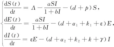
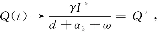
We assume that the total population is divided into five distinct epidemiological subclasses of individuals which are susceptible, latent, infectious, quarantine, and recovered (removed) with sizes denoted byS(t),E(t),I(t),Q(t) andR(t), respectively. The total population size at timetis denoted byN(t), withN(t)=S(t)+E(t)+I(t)+Q(t)+R(t).We establish the following SEIQR epidemic model of ordinary differential equations:

(1)

Summing up the five equations of system (1) and having

N′(t)=Λ-dN-(α1+k1)E-

(α2+k2)I-α3Q≤Λ-dN.

By solving the formula ofN′(t), we obtain

Thus

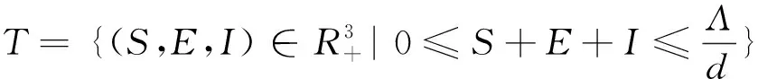
From biological considerations, we study system (1) in the following feasible region

3 Stability analysis of the disease-free equilibrium

Set the right sides of system (1) equal zero, that is,

(2)

Define

TheR0is called the basic reproduction number of system (1). It is easy to obtain the following theorem.

Theorem 3.1For system (1), there is always a disease-free equilibriumP0, and there is also a unique endemic equilibriumP*whenR0>1.

Theorem 3.2IfR0<1, the disease-free equilibriumP0of system (1) is locally asymptotically stable. IfR0>1, the disease-free equilibriumP0is unstable.

The three eigenvalues of matrixJ(P0) are

λ1=-d,λ2=-(d+p),λ3=-(d+α3+ω).

The other two eigenvalues are also the roots of the following equation:

λ2+a1λ+a2=0,

where

a1=(d+α1+k1+ε)+(d+α2+k2+k+γ),

a2=(d+α1+k1+ε)(a+α2+k2+k+γ)(1-R0).

Obviously, ifR0<1, we have the relationa2>0.Therefore, all eigenvalues of matrixJ(P0) have negative real parts. Hence, the disease-free equilibriumP0is locally asymptotically stable. IfR0>1, we get the relationa2<0.Therefore, the matrixJ(P0) has at least an eigenvalue with positive real part. Thus, the disease-free equilibriumP0is unstable.

Theorem 3.3IfR0<1, the disease-free equilibriumP0of system (1) is globally asymptotically stable.

ProofConsider the following Lyapunov function:

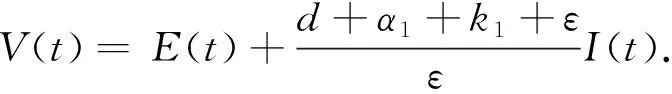
Calculating the derivative ofV(t) along the positive solution of system (1), it follows that

Furthermore,V(t)=0 only ifI(t)=0.The maximum invariant set in {(S,E,I,Q,R)|I(t)=0} is the singletonP0.The global asymptotical stability of the disease-free equilibriumP0follows from LaSalle’s invariance whenR0<1, that is, the disease-free equilibriumP0of system (1) is globally asymptotically stable.

4 Local stability analysis of the endemic equilibrium

In this section, we study the local stability of the endemic equilibriumP*(S*,E*,I*,Q*,R*) of system (1) by Routh-Hurwitz criterion theory.

Theorem 4.1IfR0>1, the endemic equilibriumP*of system (1) is locally asymptotically stable.

ProofThe Jacobian matrix of system (1) at the endemic equilibriumP*is

where

m=d+α1+k1+ε,n=d+α2+k2+k+γ.

The two eigenvalues of matrixJ(P*) are

λ1=-d<0,λ2=-(d+α3+ω)<0.

The other three eigenvalues are also the roots of the following equation:

λ3+b1λ2+b2λ+b3=0,

where

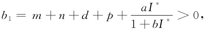
By calculation, we have

(d+p)mn+(m+n)·

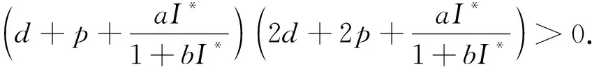
Therefore, all the five eigenvalues have negative real parts. According to the Routh-Hurwitz criterion theory, the endemic equilibriumP*of system (1) is locally asymptotically stable inDwhenR0>1.

5 The permanence of model and global stability of the endemic equilibrium

In this section, we study the global stability of the endemic equilibriumP*of system (1) by means of the periodic orbit stability theory and second additive compound matrix.

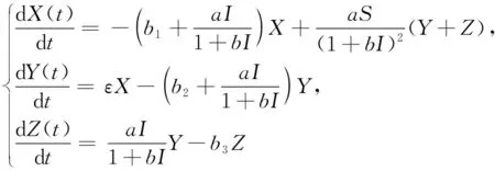
Since the first three equations of system (1) do not containQandR, using the theory of limit differential equations, system (1) is reduced to the following three-dimensional system:

(3)

Summing up the three equations of system (3) and denoting

M=M(t)=S(t)+E(t)+I(t),

having

M′(t)=Λ-dM-pS-(α1+k1)E-

(α2+k2+k+γ)I≤Λ-dM.

①Nis the largest closed invariant subset of the half-flowΦon ∂X1;

② {Nα}α∈Ais the non-cyclic coverage ofN;

③N⊂∂X1is the union of some isolated closed invariant sets;

④ any compact subset of ∂X1contains a finite number of sets of {Nα}α∈Aat most.

Then, the necessary and sufficient condition for the half-flowΦto be uniformly permanent is

whereW+(Nα)={y∈X,ω(y)⊂Nα}.

Theorem 5.1IfR0>1, system (3) is uniformly permanent.

W+(Nα)∩{T:x∈T,d(x,∂T)≤ε}=φ.

According to Lemma 5.1, system (3) is uniformly permanent aboutTwhenR0>1.

In order to study the global asymptotic stability of the endemic equilibrium (S*,E*,I*) of system (3), we first introduce the following lemmas.

Lemma 5.2[19]LetD⊂Rnbe an open set, and letx→f(x)∈RnbeC1function defined inD.We consider the autonomous system inRn.

x′=f(x)

(4)

Assume that the following conditions hold:

③ system (4) satisfies a Poincare-Bendixson criterion;

④ a periodic orbit of system (4) is orbitally asymptotically stable.

Supposex=P(t) is a periodic solution of system (4),O(x)={P(t)|0≤t≤θ} is a periodic orbit.θis period ofP(t).

Lemma 5.3[19]Consider the following system:

(5)

Consider the following Lyapunov function:

L(t)=εE(t)+(d+α1+k1+ε)I(t) ．

Calculating the derivative ofL(t) along the positive solution of system (3), it follows that

L′(t)|(3)=

ProofThe Jacobian matrix of system (3) at the disease-free equilibriumP=(S，E，I)∈Tis

Select the diagonal matrixH=diag(1,-1,1), having

For any (S，E，I)∈T, all off-diagonal elements withHJ(P)Hare non-positive, so system (3) is competitive in the areaT.

Lemma 5.6Ifp(t)=(S(t),E(t),I(t)) is a non-constant periodic solution of system (3),p(t) is asymptotically stable with an asymptotic phase orbit.

ProofSuppose thatT*(T*>0) is the period ofp(t), and calculate the second additive compound matrix of system (3) atp(t) :

where

b1=d+p+m=2d+p+α1+k1+ε,

b2=d+p+n=2d+p+α2+k2+k+γ,

b3=m+n=2d+α1+k1+α2+k2+ε+k+γ.

So as to get the second-order composite system of system (3):

(6)

Next, we prove the asymptotic stability of the zero solution of the system (6).

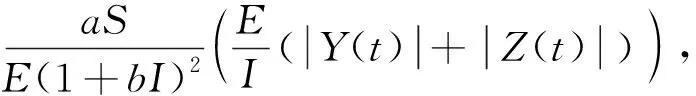
Define the norm inR3‖(x(t),y(t),z(t))‖=sup{|x(t)|,|y(t)|+|z(t)|}, consider the following function

From Theorem 5.1, there is a certain distance between the periodic solutionp(t)=(S(t),E(t),I(t)) and boundary ∂T, so there must bek>0, such that

L(t)≥ksup{|X(t)|,|Y(t)|+|Z(t)|}.

According to the relevant theory of the lower right derivative of Dini

To get

Therefore

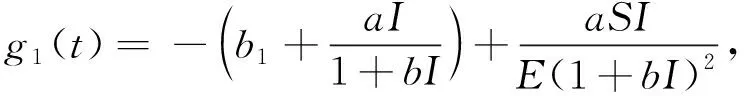
D+L(t)≤sup{g1(t),g2(t)}L(t),

where

Obtained by the system (3)

So

That is

(7)

(8)

(9)

From Equations(7), (8) and (9), whent→+∞, there isL(t)→0.Therefore, the zero solution of system (6) is asymptotically stable. From Lemma 5.3,p(t) is asymptotically stable with an asymptotic phase orbit.

By Lemmas 5.3-5.6, we know that system (3) is satisfied with every condition of Lemma 5.2. According to Lemma 5.2, we can obtain the following theorem.

Theorem 5.2IfR0>1, the endemic equilibrium (S*,E*,I*) of system (3) is globally asymptotically stable.

Theorem 5.3IfR0>1, the endemic equilibriumP*(S*,E*,I*,Q*,R*) of system (1) is globally asymptotically stable.

ProofBy Theorem 5.2, (S(t),E(t),I(t))→(S*,E*,I*), since the first three equations of system (1) do not containQandR, we obtain the following limit system of system (1):

By calculation, having

Whent→+∞, there is

Therefore, the endemic equilibriumP*(S*,E*,I*,Q*,R*) of system (1) is globally attractive in the regionD[21]. According to Theorem 4.1 , whenR0>1, the endemic equilibriumP*(S*,E*,I*,Q*,R*) of system (1) is globally asymptotically stable.

6 Example and numerical simulation

In this section, we illustrate the above-mentioned main theoretical results through numerical simulation.

Figure 1. Variational curves of S,E,I,Q and R with time t when R0=0.5531<1.

In system (1), let

Λ=0.28,d=0.02,ε=0.07,α1=0.08,α2=0.1,

k1=0.04,k2=0.08,k=0.03,γ=0.04,p=0.03.

Whena=0.08,b=0.1, by computing, we deriveR0=0.5531<1 and system (1) has a disease-free equilibriumP0(5.6,0,0,0,8.4).And we set eight initial conditions (2.6,5,2.6,1.5,2.3), (0.1,0.6,0.9,5.4,7), (2,1,1.8,3.7,5.5), (0.5,3.4,1,2.1,8), (2.5,1.5,5.2,1.8,3), (2.6,3.2,1.5, 2.5,4.2), (1.6,0.6,2.1,3.2,6.5), (5,2.7,0.6,4.2,1.5), (1,4.1,0.1,0.3,8.5), (4.3,0.7,1.5,2.7,4.8), (3.5,1.8,3.1,4.8,0.8) and (3.9,4,4.4,1.2,0.5), the numerical simulation is shown in Figure 1. From Theorem 3.3, it follows thatP0is globally asymp-totically stable. Figure 1 shows the dynamic behaviors of system (1).

Let

Λ=0.8,d=0.05,ε=0.07,α1=0.08,α2=0.1,

k1=0.04,k2=0.08,γ=0.04,p=0.03,k=0.03.

Whena=0.2,b=0.15, by computing, we deriveR0=2.3334>1 and system (1) has an endemic equilibriumP*(5.418,1.527,0.358,0.103,3.579).And we set the same initial conditions as in Figure 1, the numerical simulation is shown in Figure 2. From Theorem 5.3, we notice thatP*is globally asymptotically stable. Numerical simulation illustrates this fact in Figure 2.

Figure 2. Variational curves of S,E,I,Q and R with time t when R0=2.3334>1.

From the expression of the basic reproduction numberR0, we see that theR0depends on the prevention and control coefficientsp,k,k1andk2, and is a monotonically decreasing function of the coefficientsp,k,k1andk2(see Figure 3). Therefore, vaccination, elimination and quarantine strategies are the effective methods to control the prevalence of infectious diseases. From the expression of theR0, we also see that theR0is a monotonically decreasing function of the coefficientγ, but theR0is independent of the coefficientω.Therefore, it is also important to strengthen the non-quarantine treatment to prevent the spread of infectious diseases.

7 Conclusions

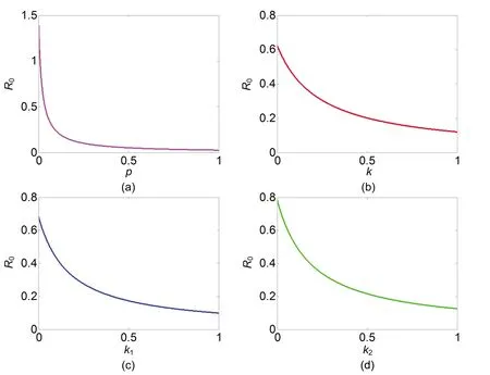
Figure 3. Variational curves of the basic reproduction number R0 with the prevention and control coefficients p, k, k1 and k2, respectively.

In this paper,we formulated an SEIQR model with saturation incidence rate and hybrid strategies, and presented a complete mathematical analysis for the global stability problem at the equilibriums of the model by means of both theoretical and numerical ways. For this model, we defined the basic reproduction numberR0which represents the average number of secondary infections from a single exposed host and infectious host. WhenR0<1, as is shown in Theorem 3.3, the disease-free equilibrium is globally asymptotically stable by Lyapunov function (see Figure 1), and the disease dies out eventually. WhenR0>1, Theorem 5.3 tells us that the unique endemic equilibrium is globally asymptotically stable by means of the periodic orbit stability theory and second additive compound matrix (see Figure 2), and the disease persists at the endemic equilibrium level if it is initially present. Finally, some numerical simulations were performed to illustrate the results.

Interestingly, the stability of the equilibrium of the model is under the influence of saturation incidence rate and hybrid control strategies. We believe that our study approaches can be applied to solve global stability problems in many other epidemic models. However, the limitation of system (1) is that it does not consider the infectious force in the latent and recovered period. However, for malaria and some other infectious diseases, the latent period and recovered period may be infectious. We leave this concern for future work.

Acknowledgments

This work is supported by Anhui Province Natural Science Research(KJ2019A0875， KJ2019A0876).

Conflictofinterest

The authors declare no conflict of interest.

Authorinformation

MaYanli(corresponding author)is currently an associate professor at Department of Common Course, Anhui Xinhua University, China. She received her MS degree in Applied Mathematics from Xi’an Jiaotong University in 2009. Her research interests include applied mathematics, biology mathematics, dynamics of infectious diseases and computer simulation.