System bias correction of short-term hub-height wind forecasts using the Kalman filter

Jingjing Xu, Ziniu Xiao, Zhaohui Lin and Ming Li

Abstract Wind energy is a fluctuating source for power systems, which poses challenges to grid planning for the wind power industry.To improve the short-term wind forecasts at turbine height, the bias correction approach Kalman filter (KF) is applied to 72-h wind speed forecasts from the WRF model in Zhangbei wind farm for a period over two years.The KF approach shows a remarkable ability in improving the raw forecasts by decreasing the root-mean-square error by 16%from 3.58 to 3.01 m s−1, the mean absolute error by 14% from 2.71 to 2.34 m s−1, the bias from 0.22 to − 0.19 m s−1,and improving the correlation from 0.58 to 0.66.The KF significantly reduces random errors of the model, showing the capability to deal with the forecast errors associated with physical processes which cannot be accurately handled by the numerical model.In addition, the improvement of the bias correction is larger for wind speeds sensitive to wind power generation.So the KF approach is suitable for short-term wind power prediction.

Keywords: Wind forecasts, Wind energy, Numerical model, Bias correction, Kalman filter, Atmospheric boundary layer

1 Introduction

Wind energy is one of the most important sources of renewable energy, and over the last decade there has been rapid growth in wind energy production in China.Because of its stochastic nature, wind is inherently varying and wind energy is a fluctuating source for power systems [1].Accurate wind power prediction can reduce the risk of uncertainty and lead to better grid planning and integration of wind energy.Thus, short-term wind power prediction, which has been discussed widely [2–5], is useful in power system planning.According to the demands of the wind energy industry, 15-min wind speed forecast at turbine height with a forecast period of 24–72 h should be provided for short-term wind power prediction.

Numerical weather prediction (NWP) models can exhibit systematic errors in wind speed and ramp event forecasts [6–8], especially near the surface.This can be caused by many factors, such as shortcomings in the physical parameterization, inability to successfully handle sub-grid phenomena, inaccurate initial and lateral boundary conditions, interpolations to areas not close to grid points or model levels, and smoothed orographic and landscape characteristics associated with the model horizontal resolution.To reduce the influence of these drawbacks in the final output of a NWP model, a variety of approaches based on statistical methods have been used [9–11], such as linear regression, moving average correction, partial least squares method, etc.These approaches are called model output statistics (MOS)methods, and employ postprocessing bias correction to improve the direct model outputs.

One of the most convenient postprocessing approaches is Kalman filter (KF) [12], which is a statistically optimal sequential estimation procedure for dynamic systems.Observations are recursively combined with recent forecasts using weights that minimize the corresponding biases.The KF approach carries minor computational costs and can easily adapt to any alterations in observations.In addition, this recursive and adaptive method does not need an extensive database for training.

The KF method has been widely used for improving weather forecasts of continuous variables such as 2 m temperature, 10 m wind speed and ozone concentration etc.[13–17].As a postprocessing bias correction method,the KF uses recent past observations and forecasts to estimate the model bias in future forecasts to correct the raw forecasts.The nonlinear formation of Kalman filter has been applied to improve short-term wind speed forecasts at turbine height [18] and to forecast wind speed and wind power at a wind farm site [19].Reference[20] modifies the nonlinear Kalman Filter proposed in[18] and applies the method to improve the wind ramp event forecasts for wind power industry.As well as the MOS methods and the KF approach, many studies have employed various other approaches to improve shortterm wind speed and power forecasts, such as analog bias correction [21, 22], Gaussian process regression [23],machine learning techniques such as neural network [24,25] and random forests [21], analog ensemble [26] and time-dependent bias correction [27] for probability forecasting.Other related studies include data preprocessing technique [28] and circular-circular regression method for wind direction forecasts [29].

Reference [30] shows that in the lower atmosphere,forecast errors can be correlated for several days and contain strong diurnal variability.So in this paper, diurnal behavior of the forecast error is taken into consideration and the KF is applied to Zhangbei wind farm in northeastern China to perform a detailed statistical analysis.The state-of-the-art MOS method is also employed as a comparison to evaluate the forecast skill of the KF approach.The discussion is focused on the capability of the KF to improve the raw forecasts, especially on systematic and random errors.

The rest of this paper is organized as follows.In Sect.2,information on the wind farm, the WRF model and the experimental design is provided.Since the turbine height (60–100 m) is in the lower boundary layer, a special Kalman filter for each hour of the day is presented in Sect.3, so that the forecast error can be estimated from data with lags of multiple of 24-h.In Sect.4 a case study on wind speed forecasts in Zhangbei wind farm over two years is illustrated.Finally, Sect.5 draws conclusions.

2 Wind speed datasets and numerical simulations

2.1 The wind farm and observations

Zhangbebi wind farm is located northwest of Hebei Province in China.The farm consists of 66 wind turbines with a total installed capacity of around 100 MW.The wind turbine height is 70 m, and the wind farm covers complex mountain terrain with the altitude ranging from 1600 to 1800 m (see Fig.1).

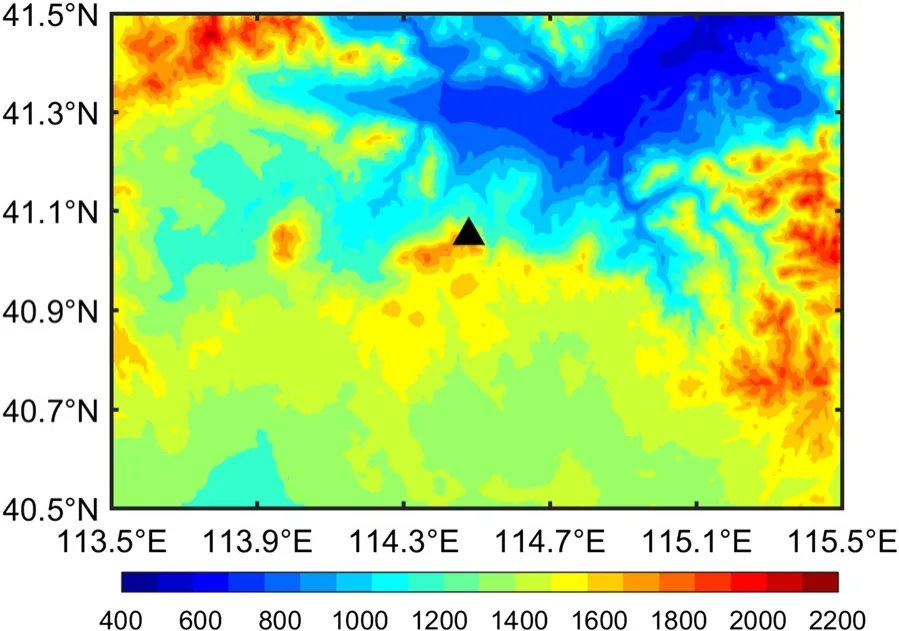
Fig.1 Location of Zhangbei wind farm (the black solid triangle denotes the observation station)

Observational data comes from one mast situated at the wind farm, at latitude 41° 03′ N, longitude 114° 29′ E and altitude 1660 m.Wind speed data was recorded by the anemometer with a sampling rate of 5 min.The dataset used in the present study spans over 2 years, from 07 November 2015 to 22 February 2018(839 days in total), and the measurements are averaged over 15 min in order to meet the demands of the wind power industry.

2.2 The WRF model and experimental design

The WRF model is a nonhydrostatic compressibleequation, mesoscale NWP model [31], and the proposed bias correction methods have been applied to improve the hub-height wind speed forecasts provided by the WRF model.

In the present study, the WRF model is run over northeastern China with three nested domains centered on Zhangbei wind farm with 27-km, 9-km, and 3-km horizontal grid increments.The forecast periods are 24-h, 48-h and 72-h, and the wind speeds are issued in 15-min increments.Vertical levels in the model have fine resolution around wind turbine height with 48 levels in total and 6 levels in the lowest 100 m.The 70-m wind speed forecasts within the finest domain are bilinearly interpolated to the observation location directly.The parameterizations chosen for these experiments include the Purdue Lin microphysics scheme, the Mellor–Yamada–Janjic planetary boundary layer (PBL)scheme, the Eta scheme for the surface layer, the Kain–Fritsch scheme for the convective processes (only in the two coarser domains), and the Noah land surface model for the land surface scheme.

3 Bias correction procedure

3.1 The Kalman filter (KF) approach

In numerical weather forecasts, the specific KF approach predicts the future bias as equal to the old bias plus uncertainty, which is corrected by the linear function of the difference between the previous prediction and verifying bias.

In our study, the KF method models the true(unknown) forecast bias xtat timetby the previous true bias plus a white noise wtterm as:

thus, ytincludes both the systematic bias and random error.Therefore, the system matrix and the observation matrix are designated as the identity matrix for the proposed algorithm.The random vectors wtand vtmust follow the normal distribution with zero mean and be independent.

Kalman [12] showed that the optimal recursive predictor of xtcan be written as a combination of the previous bias estimation and the previous forecast error.The optimal estimates given for the state vector xtand covariance matrix Ptat timetare:

As soon as the new value ytbecomes known, the new value of state vector xtis calculated as:

where Ktis the Kalman gain matrix and is the most crucial parameter of the filter.Ktdetermines how easily the filter will adjust to any possible new conditions, and is given as:

Finally, the new value of the covariance matrix Ptof the unknown state is given by:

Equations (3)–(6) are known as updating equations,which update the Kalman algorithm from time t −t tot.Note that − 1 denotes the inverse matrix while I stands for the identity matrix.This procedure is recursive because values of the KF coefficients at any one-time step depend on the values at the previous time step, and it is optimal in a least-squares sense.

Since xtand Ptconverge to their true values rapidly,the initial values x0, P0do not seriously affect the results of the algorithm.However, the way in which the covariant matrices Wtof the random vector wtand Vtof vtare calculated during the process can significantly affect the final outcome.In our case, the system covariant matrix Wtand observation covariant matrix Vtare estimated based on the samples of the last 7 values of wt= xt−xt-1and vt= yt−xtrespectively, as:

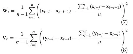
wheren= 7 andn− 1 represents unbiased estimation.The period of 7 values has proved to be the optimal choice in the study for successful correction and fast adaptability.Here the initial values of xt, Pt, Wtand Vtare set to 0, 4, 1 and 6, respectively.

Because the original data is in 15-min increments, the observations and forecasts are transformed to one-hour averages as pre-processing of the bias correction.The results for the first 39 days are removed to eliminate the effects of the KF algorithm’s spin-up, and the results for the remaining 800 days are then analyzed.Finally, the corrected one-hour wind speeds are transformed back to 15-min wind speeds.

3.2 Model output statistics (MOS) method

Since the MOS method is the most widely used in postprocessing techniques for numerical models, the correction results by the MOS method are also provided to compare with the KF correction results.

MOS uses a multiple linear regression to correct systematic errors in NWP models using NWP outputs of certain weather variables as predictors and fitting these predictorsto observations.To find the optimal predictors, the MOS multivariate regression equations are used.

MOS aims at correcting forecasts by means of a regression functionrbetween the variableYto be predicted and some explanatory variable(s) (or predictors)Xwhich may be NWP model output(s) or any other source of information.This regression function is estimated based on past forecasts and associated observations, and it is then applied to future forecasts to increase their accuracy.In the present study, a classical regression method is applied [32], and the regression function is a second-order polynomial relationship of the explanatory variables as:

whereβ0is a real number,βis a vector of real numbers,and X1,2is the vector containing every possible combination of product of explanatory variables of order 1 and 2(called interactions).The parametersβ0andβare fitted onto the training dataset with an ascending selection of predictors based on the Bayesian information criterion.WRF-modeledU,V, andWwind components, wind speed (wspd), temperatureT, pressurePand relative humidity (rh) are used as potential predictors here.

4 Results and discussion

The bias correction methods presented in Sect.3 are applied to improve the wind speed forecasts in this section.The root-mean-square error (RMSE) can be decomposed as:

where

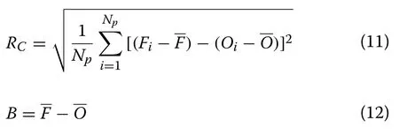
In Eqs.(10)–(12), the variableRrepresents RMSE,RCrepresents the centered root-mean-square error(CRMSE), andBdenotes bias.Oiis the observation value at timeiandFiis the corresponding forecast value.Npis the size of sample which means the number of pairs (Fi,Oi).and O are the mean forecast value and observation value, respectively.CRMSE is considered to be the random component of RMSE, while the systematic component is represented by bias.CRMSE can be associated with the intrinsic predictive skill of the forecast because of the limitation of physical parameterization, and bias estimates the systematic errors which may be associated with biased initial conditions, smoothed topography, offset parameter values, etc.

4.1 Global performance

To evaluate the performance of the bias correction, the global metrics of the results are investigated first.Table 1 characterizes the ability of improving forecast skill for the bias correction quantitatively, based on metrics of bias,mean absolute error (MAE), RMSE, CRMSE and the correlation coefficient.Because the study mainly analyzes the bias correction results for 72-h forecasts, only 72-h MOS bias correction results are presented as comparison.From Table 1, it can be seen that the KF approach for 72-h forecasts has decreased RMSE by 16% from 3.58 to 3.01 m s−1, MAE by 14% from 2.71 to 2.34 m s−1, bias from 0.22 to − 0.19 m s−1, and improved the correlation from 0.58 to 0.66.The result for CRMSE is similar to that for RMSE.Table 1 also shows the results of the KF bias correction for 24-h and 48-h forecasts.It is not surprising that the KF for 24-h forecast shows the best performance,as when the forecast period gets longer, the correction effect is weakened.For results of 24-h forecasts, the KF bias correction has decreased RMSE by 18%, MAE by 16%, bias by 27%, and improved the correlation from 0.58 to 0.67, with all the metrics showing remarkable improvement.Although 0.6 m s−1improvement in RMSE in some circumstances is not seen to be high, this is a substantial improvement in wind energy.In a 2008 Department of Energy publication, it was stated that, “a 1% error in wind speed estimates for a 100-MW wind generation facility can lead to losses approaching $12,000,000 over the lifetime of that plant” [33].The MOS bias correction also shows moderate improvement, decreasing RMSE by 10%,MAE by 8% and bias by 14%.From the above results, it is obvious that the KF is suitable for short-term wind power prediction with the forecast period of 24–72 h.In the rest of this paper, only the results for 72-h forecast are analyzed as representative forecasts.

Table 1 The overall performance of the KF bias correction for 24-h, 48-h, 72-h forecasts and MOS bias correction for 72-h forecasts based on the five metrics (bias, MAE, RMSE, CRMSE, and correlation coefficient)

Table 2 The overall performance of the KF and MOS bias corrections for wind speeds sensitive to wind power prediction based on four metrics (bias, MAE, RMSE, and CRMSE)

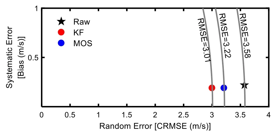
Fig.2 Bias (m s−1) as a function of CRMSE (m s−1), showing the raw forecasts and the KF and MOS bias corrections

From the relationship shown by (10), if CRMSE is plotted against the bias, the distance of the point from the origin is equal to RMSE.Figure 2 illustrates such a diagram for the raw forecasts and the KF and MOS bias corrections, where the radial distances from the origin to the gray circular lines equal RMSE.Obviously, wind speed errors in this forecast system are dominated by the random component.The KF not only reduces the bias component of RMSE, but also the remaining part.The latter can be seen as the ability of the KF to add predictive skill to the raw forecasts by reducing random errors.

4.2 Seasonal and diurnal variability for bias correction

To investigate the seasonal and diurnal characteristics of the forecast errors, the two metrics with all the available data at a given time of the 24 forecast hours are computed.Figures 3 and 4 show the temporal evolution of bias and CRMSE, respectively for the raw forecasts, and the KF and MOS bias correction results.

The biases in summer and autumn are much larger than in winter and spring, and exhibit violent diurnal variation.The maximum bias is almost 3 m s−1which appears in summer.The growth of the planetary boundary layer (PBL) is often a challenging process for prediction, which is reflected by the jump in the bias values before sunrise (05 LST-07 LST) in summer and autumn(Fig.3).Throughout the daytime and early evening, the bias values stay constant around 0.5 m s−1, and before sunrise, the raw forecasts show an increase in bias, given the uncertainty associated with the PBL growth.The KF shows improvement across all the forecast hours in the range of 0.5–2.5 m s−1with respect to the raw forecasts,while decreasing bias around 1.5–2.5 m s−1in 05 LST-07 LST.This is the indication of the KF method’s ability to improve the predictive skill.In winter and spring,the diurnal cycles are not so obvious compared to those in summer and autumn, and the KF correction effect is not so remarkable.The MOS bias correction also shows moderate improvement in summer and autumn, especially in PBL growth time, though the KF approach performs better than the MOS method nearly all the time.

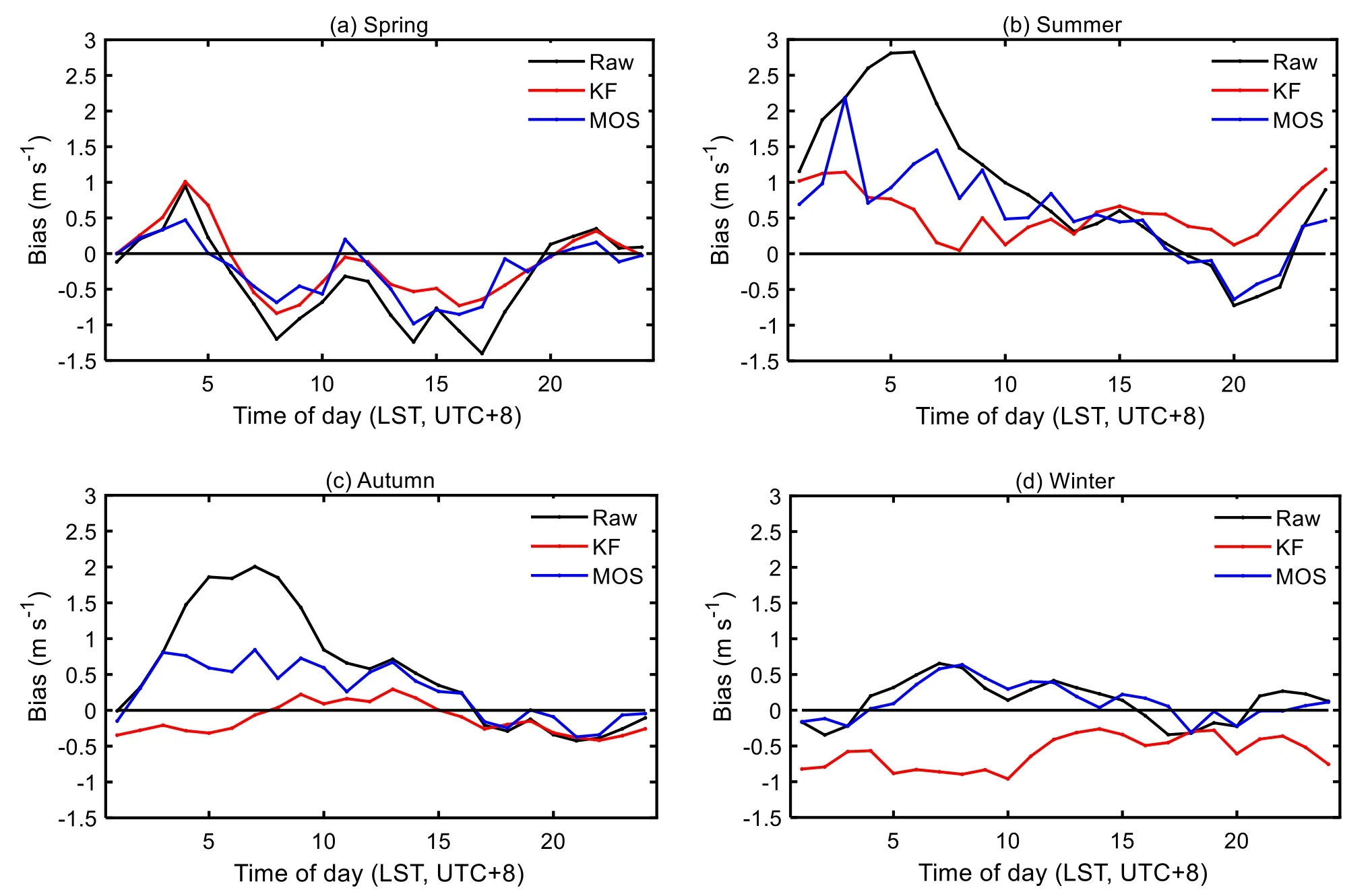
Fig.3 Temporal evolution of bias in a spring, b summer, c autumn, d winter for the raw forecasts, and the KF and MOS bias corrections across the 24 h of forecast

For CRMSE (Fig.4), the results are contrary to those for bias.The CRMSE in winter and spring is larger than in summer and autumn, and the maximum CRMSE appearing in winter is almost 4.5 m s−1.The KF drastically reduces CRMSE of the raw forecasts by 1 m s−1in winter.In spring, there is a high peak around 09 LST-10 LST, and then it drops abruptly by almost 1.5 m s−1.The KF approach reduces CRMSE by around 1 m s−1in this time interval, showing the capability to handle the forecast error associated with PBL growth.Figure 4b shows similar results in summer.The KF reduces CRMSE of 0.7–1.0 m s−1from midnight to noon.The MOS method shows little improvement for CRMSE in all four seasons, which indicates that the MOS method mainly reduces bias of the forecast error rather than the CRMSE component.

Fig.4 Temporal evolution of CRMSE in a spring, b summer, c autumn, d winter for the raw forecasts, and the KF and MOS bias corrections across the 24 h of forecast

4.3 Evaluation of wind speed forecasts sensitive to wind power prediction

It is well known that wind speed forecasts for wind power prediction are different from routine wind speed forecasts according to the wind turbine power curve.When wind speed is equal to or less than 5 m s−1a turbine will not generate power output, while once the wind speed exceeds 12 m s−1, the wind turbine reaches its maximum capability.So forecast accuracy for wind speed between 5 and 12 m s−1is essential to wind power prediction.Hence the wind speed forecasts sensitive to power prediction are evaluated in this subsection.

Figure 5 gives the wind speed distribution of the observation, the raw forecasts, and the correction.For the KF approach (Fig.5a), the bias correction mainly improves the raw forecasts in 4–12 m s−1, except for wind speeds in the 5–7 m s−1interval.In the wind speed interval of 9–12 m s−1, which are included in the area sensitive to wind power prediction (5–12 m s−1), the correction shows significant efficiency.While for the MOS method(Fig.5b), the bias correction only provides small improvements on the raw forecasts in most wind speed intervals.

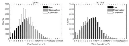
Fig.5 The wind speed distribution of the observation, the raw forecasts and the a KF, b MOS

To quantitatively evaluate the performance of the two bias correction methods for wind speeds sensitive to wind power prediction, the results are presented in Table 2.The raw forecasts for wind speed sensitive to wind power show better forecast skill than in Table 1 based on all four metrics.This is rational because the model exhibits large errors when wind speed is low.In complex terrain, low wind speed is always associated with local circulations which cannot be accurately handled by the numerical model.The KF has decreased RMSE by 18% from 2.91 to 2.40 m s−1, MAE by 17% from 2.28 to 1.88 m s−1.The larger reduction of CRMSE by 19% from 2.90 to 2.36 m s−1compared to RMSE, is due to the promoted bias.Thus, for wind speeds sensitive to wind power, the improvement of the bias correction is larger.This result proves that the KF approach is especially suitable for wind power prediction.The same fact can be seen in Fig.6, while the MOS method also shows moderate improvement for wind speeds sensitive to wind power prediction.

Fig.6 Bias (m s−1) as a function of CRMSE (m s−1) for wind speeds sensitive to wind power prediction, showing the raw forecasts, and the KF and MOS bias corrections

The overall performance of the two bias correction methods has been evaluated.In contrast to MOS and other statistical methods which require a long training period and behave in a static manner, the KF approach adapts its coefficients during each time step.It requires a much shorter training period, and can adapt to changing synoptic conditions, changing seasons, and even changing weather forecast models.However, the disadvantage of the method is that it is less likely to predict extreme bias events, e.g., it is unable to anticipate a large bias when all biases for the past few days have been small.

5 Conclusions

To improve the short-term hub-height wind speed forecasts for wind power prediction, a postprocessing bias correction Kalman filter approach is applied to 72-h wind speed forecasts at 70-m height from the WRF model in Zhangbei wind farm for a period of more than two years.The main conclusions can be summarized as follows:

The KF approach for 72-h forecasts has decreased RMSE by 16% from 3.58 to 3.01 m s−1, MAE by 14%from 2.71 to 2.34 m s−1, bias from 0.22 to − 0.19 m s−1,and improved the correlation from 0.58 to 0.66.Wind speed errors in this forecast system are dominated by the random component, while the KF not only reduces systematic errors of the model, but also significantly reduces random errors of it.

In all seasons, the forecast errors (including systematic errors and random errors) of the raw forecasts exhibit a strong diurnal cycle with a peak before sunrise in PBL growth time.The KF approach significantly reduces random errors of the model when the PBL growth occurs, showing the capability to deal with the forecast errors associated with physical processes which cannot be accurately handled by the numerical model.In contrast, the MOS method mainly reduces systematic component of the error rather than the random component.

The improvement of the KF is larger within the range of the power curve where power generation is most sensitive to wind speed.This fact shows that the KF approach is especially suitable for wind power prediction.And with the advantages of shorter training periods and faster adaption time than traditional statistical methods, the KF approach is suitable for short-term wind power prediction with the forecast period of 24–72 h.

Abbreviations

NWP: Numerical weather prediction; MOS: Model output statistics; KF: Kalman filter; WRF: Weather Research and Forecasting; PBL: Planetary boundary layer; RMSE: Root-mean-square error; CRMSE: Centered root-mean-square error; MAE: Mean absolute error; LST: Local standard time; UTC: Coordinated universal time.

Acknowledgements

Not applicable

Authors’ contributions

JJX performed the study of the experiments and conducted the draft of the manuscript, ZNX the corresponding author, engaged in modifying the paper and submitted it to the PCMP.ZHL and ML checked the grammar and writing of the paper.All authors read and approved the final manuscript.

Funding

This research was supported by National Key R&D Program of China(Technology and application of wind power/photovoltaic power prediction for promoting renewable energy consumption, 2018YFB0904200) and eponymous Complement S&T Program of State Grid Corporation of China(SGLNDKOOKJJS1800266).

Availability of data and materials

The datasets generated and analyzed during the current study are not publicly available because the dataset of the target wind farm is confidential.

Declarations

Competing interests

The authors declare that they have no known competing financial interests or personal relationships that could have appeared to influence the work reported in this paper.