Linearization threshold condition and stability analysis of a stochastic dynamic model of one-machine infinite-bus(OMIB)power systems

Lijuan Li,Yongdong Chen,Bin Zhou,Hongliang Liuand Yongfei Liu

Abstract With the increase in the proportion of multiple renewable energy sources, power electronics equipment and new loads, power systems are gradually evolving towards the integration of multi-energy, multi-network and multisubject affected by more stochastic excitation with greater intensity.There is a problem of establishing an effective stochastic dynamic model and algorithm under different stochastic excitation intensities.A Milstein-Euler predictorcorrector method for a nonlinear and linearized stochastic dynamic model of a power system is constructed to numerically discretize the models.The optimal threshold model of stochastic excitation intensity for linearizing the nonlinear stochastic dynamic model is proposed to obtain the corresponding linearization threshold condition.The simulation results of one-machine infinite-bus (OMIB) systems show the correctness and rationality of the predictorcorrector method and the linearization threshold condition for the power system stochastic dynamic model.This study provides a reference for stochastic modelling and efficient simulation of power systems with multiple stochastic excitations and has important application value for stability judgment and security evaluation.

Keywords: Power system stability, Stochastic dynamic model, Stochastic excitation, Stochastic processes, Threshold condition

1 Introduction

Driven by energy reform and emerging technologies, the trend of the “three highs” (high proportion of renewable energy source grid connection, high proportion of power electronics equipment and high proportion of new loads)and “three multiples” (multiple energy sources, multiple networks and multiple subjects) in smart grids is gradually accelerating [1].This not only creates huge economic benefits for power systems but also brings large numbers of random factors to the systems.The input of a large number of random factors is a new challenge for safety and stability [2, 3].The system security problems caused by random factors have been of considerable concern to the industry [4, 5].The establishment of an effective power system stochastic dynamic model and algorithm is the basis for a system safety and stability analysis influenced by random factors [6].

Although there always existed random factors in power systems, in the past they have not become important factors affecting the safe and stable operation of the system, and thus were usually ignored.With the increase of new energy penetration and the proportion of new load access, the random factors have become the key factors influencing security and stability, and can no longer be ignored.Random factors are mainly made up of three types, i.e., randomness of the initial values, of parameters and of external excitations [7].The randomness of the initial value is caused by a change of power flow before and after the power system is disturbed.The randomness of parameters is caused by the changes of operating state and internal topology of the equivalent model.The causes of external excitation randomness include the randomness of new energy power generation, of network events, of variable loads and of external interference in regional interconnected power grids etc.In a certain dynamic process of a power system, the randomness of the initial values and parameters are considered constants, and these can be examined using probability methods.However, the randomness of external excitations changes rapidly and is time-varying in the dynamic process, and thus stochastic differential equation theory is necessary for modelling and analysis [8, 9].

In a power system, a stochastic differential equation can accurately describe the dynamic process and operational characteristics of the system and establish a more realistic stochastic dynamic model of the power system[10].Based on the deterministic model,random variables describing random factors of the system are usually introduced to establish the stochastic dynamic model of a power system to study its stability [11].In the process of operation, the dynamic process of external excitation is considered to be a stochastic process.In much engineering practice, external stochastic excitation is generally considered Gaussian white noise with a stable independent increment and zero mean value [12], and a linear stochastic dynamic model of a power system is used to conduct the relevant research [13–15].However, actual power systems are multi-dimensional complex and nonlinear dynamic systems [16].When the stochastic excitation intensity near a node in the system is relatively large, the results obtained using a linear stochastic dynamic model for analysis may have relatively large errors.Therefore, it is necessary to use a nonlinear stochastic dynamic model of the power system [17–19],one which can describe the dynamic process of the system more aptly.The stability of the system can be analyzed by using the nonlinear stochastic dynamic model for more accurate conclusions.

The solution of a stochastic dynamic model of a power system is the premise of system stability analysis.However, in general, it is difficult to obtain the analytic solutions of stochastic differential equations and only under some special circumstances can the exact analytic solution expression be obtained [20].Therefore,an appropriate numerical method is constructed to obtain the trajectory of the solution process so as to approximate the true solution [21, 22].Commonly used numerical methods for solving linear and nonlinear stochastic differential equations include the Euler-Maruyama [23],Milstein [24], and Runge-Kutta methods [25], etc.Among them, the predictor-corrector algorithm for stochastic differential equations is not only easy to calculate but also has high stability [26], and is thus suitable.The method has a simple solution process and high computational efficiency for the linear case, but it also has a complex solution process and low computational efficiency in solving nonlinear stochastic dynamic models.In [13], a nonlinear model is approximately converted to a linear model to reduce the complexity of the subsequent solving.However,the linearization process ignores the influence of the nonlinear characteristics of the system, so stability analysis deviation will occur when the stochastic excitation of a power system increases.

A stochastic small disturbance generally refers to the fluctuations of loads and parameters (such as the switching of small-capacity load).Because of the small stochastic excitation, the stability analysis of a system with such small disturbances is often approximated by linear models, and the methods include the Monte Carlo and stochastic response surface methods.A stochastic large disturbance is a sudden change of large-capacity load(such as switching of large-capacity load, switching of main system components, or component failure).For such a large disturbance, a nonlinear model is needed,and its stability analysis methods include the extended equal area and pseudo-Hamiltonian system stochastic average methods [1].With the increase of new energy penetration, grid-friendly load and flexible load ratio(double highs), stochastic factors and stochastic excitation intensity increase.Stochastic excitation intensity caused by load and parameter fluctuations may become a large disturbance.Under such conditions, the distinction between a stochastic small and large disturbance is no longer clear.This brings difficulties to the choice of linear or nonlinear models for the analysis.Most existing studies focus on the stochastic excitation threshold indicating whether or not the system is unstable [27].Therefore, it is necessary to study the stochastic excitation intensity thresholds of the linear and nonlinear models.

For a power system under the action of stochastic excitations of different intensities, this paper studies the stochastic excitation threshold conditions that can be used to linearize a nonlinear stochastic dynamic model and select the stochastic dynamic model of the power system, while ensuring the accuracy of both the model and solution.Furthermore, the influence of the stochastic dynamic model linearization on stability analysis is analyzed quantitatively.

The main contributions of this paper can be summarized as follows.(1) The Milstein-Euler predictorcorrector method for power system stochastic dynamic models is constructed.This improves the stability of the algorithm and provides new ideas for solving the stochastic dynamic models.(2) A threshold discrimination basis for linearizing nonlinear power system stochastic dynamic models is proposed.This avoids the deviation of stability analysis caused by the linear model solution method when the linearization condition of the stochastic dynamic model is not satisfied.It shows the influence of different stochastic excitation intensities on model selection and stability analysis, and provides a reference for power system stochastic modelling and efficient simulation.

The rest of the paper is organized as follows.The stochastic dynamic model of a power system is established in Section 2 and the Milstein-Euler predictor-corrector method is described in Section 3.The stability of the predictor-corrector method is analyzed in Section 4, the optimal threshold model of stochastic excitation intensity is established and its stability is analyzed in Section 5.The threshold value of stochastic excitation intensity is determined, and the stability of stochastic excitation intensity above and below the threshold value is analyzed in Section 6.Finally,the paper is concluded in Section 7.

2 Stochastic dynamic model of power systems

2.1 Nonlinear stochastic dynamic model of power systems

A stochastic dynamic model of a power system is constructed by adding a stochastic excitation term based on a deterministic model.To simplify the calculations, improve operational efficiency and eliminate the interference of other factors in drawing correct conclusions, the most representative OMIB system is often used for modelling and analysis [28].In such a system, the deterministic model is an equation describing the rotor motion as:

where Pe=E’Usinδ/X∑, Pm=Pe(0)=E’Usinδ0/X∑, M, δ,D, Pe, Pm, E’, and δ0are the inertia time constant, power angle, damping coefficient, electromagnetic power,mechanical power, internal potential and initial power angle of the generator respectively.t is time, U is the infinite bus voltage and X∑is the total reactance of the system.Assuming Pmis constant, it can be seen from the steady-state power balance condition that its value is equal to the steady-state value of Pe.

Power fluctuation in a power system caused by external stochastic excitation such as new energy generation and load fluctuates around a certain mean value in a relatively short time.This can be regarded as a Gaussian white noise process with a stable independent increment [12].Therefore,a stochastic excitation item is added to the right side of(1)to construct the stochastic dynamic model,as:

where σ is the stochastic excitation intensity and W(t) is the stochastic excitation modelled as a standard Gaussian white noise process.Stochastic excitation is generally regarded as the stochastic fluctuation of new energy generation power, load, etc.

The general stochastic differential equation is driven by Brownian motion (also called the Wiener process),while the stochastic dynamic model in this paper is driven by Gaussian white noise.Therefore, it is necessary to convert Gaussian white noise to the form of Brownian motion to establish the final differential equation model.From stochastic differential equation theory,the derivative of Brownian motion B(t) is characterized by Gaussian white noise, as:

According to (3), the nonlinear stochastic dynamic model of the power system is obtained as [19]:

where ω and ω0are the generator speed and its initial value respectively.The vector form of(4) is:

Because (5) presents strong nonlinear characteristics,it is difficult to find its analytic solution.

2.2 Linearization of stochastic dynamic model of power systems

By linearizing (4), a linear stochastic dynamic model of the power system is obtained as [13]:

The corresponding vector form of (6) is:

The explicit expression of the analytic solution of (7)is:

3 Algorithm construction

3.1 Construction of predictor-corrector methods for a nonlinear stochastic dynamic model

For the nonlinear stochastic dynamic model of the power system shown in (5), the Milstein-Euler predictor-corrector method is constructed to carry out the numerical discrete process of the model as follows.

Use the explicit Milstein method to obtain the predictor scheme, as:

Use the implicit Euler method to get the corrector scheme:

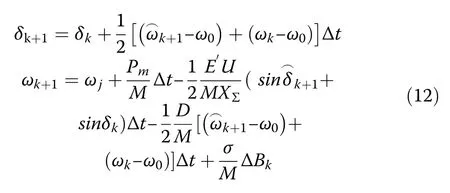
where n=1,2, …,L, Δt=T/L, ΔBn～(√Δt)N (0,1), and N(0,1) is the standard normal distribution.For a positive integer N*, Δt=T/N*, tk=kΔt, δk=δ (tk), ωk=ω (tk), and k=0,1,2, …,K.The specific coefficients in (5) are substituted into (9) and (10) to yield its predictor scheme:

and its corrector scheme:

3.2 Construction of predictor-corrector methods for linear stochastic dynamic model

For the linear stochastic dynamic model shown in (7),the Milstein-Euler predictor-corrector method is constructed to carry out the numerical discrete process of the model as follows.

Use the explicit Milstein method to get the predictor scheme,i.e.:

Use the implicit Euler method to get the corrector scheme:

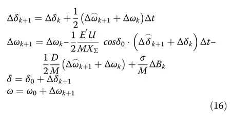
where n=1,2, …,L, Δt=T/L, ΔBn～(√Δt)N (0,1), and N(0,1) is the standard normal distribution.For a positive integer N*, Δt=T/N*, tk=kΔt, δk=δ (tk), ωk=ω (tk), and k=0,1,2, …,K.The specific coefficients in (7) are substituted into (13) and (14) to obtain its predictor scheme:

and its corrector scheme:

4 Algorithm stability analysis

According to (5) and (7), the coefficients (F(X(t)), AX(t))and (G(t), Q(t)) respectively satisfy the consistent Lipchitz condition and linear growth condition [29], as:

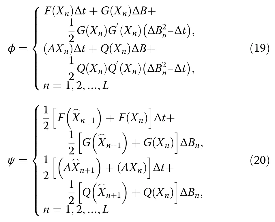
where ∨represents the OR operation,L1and K1are both normal numbers, and the absolute values of the derivative of G(t) in (5) and Q(t) in (7) are less than the constant M0.The increment functions ϕ and ψ of the Milstein-Euler predictor-corrector method in (9), (10),(13) and (14) are:

while ϕ and ψ meet the following conditions:

where C1, C2, C3, C4, K2and K3are all normal numbers,while C1=L1, C2=(6+3 M0/4) L2 1, C3=L1/2, C4=2 L2 1, K2=(6+3 M0/4) K2 1 and K3=4.ξ1, ξ2, η1and η2are arbitrary real numbers, while Iϕand Iψare the integral form of It.Note (1): M0: G(t) (0 and σ/M) in (5) and Q(t) (0 and σ/M) in (7) are constants, and the absolute values of their derivatives are zero.Thus, M0can be any constant greater than zero.The left side of the inequality in (17) is an OR operation.G(t) in (5) and Q(t) in (7) are constants, and subtracting the two equals zero.Thus, L1can be any constant greater than zero.Similarly, the left side of the inequality in (18) is also an OR operation.G(t) in (5) and Q(t) in (7) can take the values of zero and σ/M.Therefore, K1can be any constant greater than σ/M.

In summary, the power system stochastic dynamic model established in this paper satisfies the conditions in (21) to (26), so the Milstein-Euler predictor-corrector method in (9), (10), (13) and (14) is mean square zero stable, that is, the constructed predictor-corrector methods suitable for the power system are also mean square zero stable.Although common numerical methods such as Euler-Maruyama, Milstein, and Runge-Kutta are mean square stable, the Milstein-Euler predictor-corrector method constructed in this paper is more stable than the above-mentioned methods.

5 Optimal threshold model and stability analysis

5.1 Optimal threshold model of stochastic excitation intensity

Converting a nonlinear stochastic dynamic model to a linear stochastic dynamic model results in certain errors,and the linear conversion of a nonlinear stochastic dynamic model is only effective when the error is controllable.To obtain the discrimination basis of the effectiveness indication of the linearization of a nonlinear stochastic dynamic model, we establish the optimal threshold model of stochastic excitation intensity.This can be linearized by the nonlinear model according to stochastic dynamic models in (5) and (7).The stochastic excitation intensity threshold for effective linearization of the model is the maximum allowed within the controllable error range.Beyond this threshold, the error will exceed the allowable range and the linearization of the model is no longer effective.When the intensity does not exceed the threshold, the nonlinear model can be linearized and the stability of the system can be analyzed using the linear model.Therefore, within the controllable error range, the objective function of the optimization model is:

where Xnot(t) and X(t) are the outputs of the state variables δ of the nonlinear and linear models respectively,while |Xnot(t)-X(t)| is the error between the two models.Through optimization, the error is maximized, and the corresponding stochastic excitation intensity threshold σcis obtained.

The constraints of this optimization model are:

Equations (28) and (29) are the nonlinear and linear models respectively, that is, the stochastic differential equation constraints corresponding to σ.Δδeris the power angle error between Xnot(t) and X(t) (the error cannot exceed Δδc).

Note (2):The values of Δδervary due to different operating conditions, application scenarios, research goals and error accuracy requirements.Accurate calculation and analysis in a power system are conducive to system security, stability and control.Therefore, when selecting the upper boundary of error, the proposed method allows the transformed linear system to fit the nonlinear system and accurately describes the actual operation of the system.By adjusting the upper bound of error, the threshold model can also be applied to the stability analysis of small and large interference.The specific basis for setting the upper error boundary will be further discussed in the follow-up research.

The objective function and constraints can be expressed as the following constrained optimization problem:

Under the constraints, the objective function is maximized to obtain the optimal threshold of stochastic excitation intensity.The specific steps for solving the optimal threshold model of the intensity are as follows.

1) Input a set of values of stochastic excitation intensity σ,and solve the output of the state variables δ corresponding to the constraints (28)and (29) according to (11),(12),(15) and (16).

2) With the above-mentioned σ, calculate the error of the state variable δ corresponding to (28) and (29),namely Δδer.

3) Under constraint (30), the grid search method is used to obtain the σ corresponding to (28) and (29).

4) Repeat the above 3 steps until the maximum stochastic excitation intensity within the error range is obtained.This is the intensity threshold σc.

The threshold of stochastic excitation intensity σcis thus obtained.When σ ≤σc, the nonlinear stochastic dynamic model is linearized and the stability of the system is analyzed using the linear stochastic dynamic model to reduce computational complexity and improve simulation efficiency.The nonlinear stochastic dynamic model is used to analyze the stability of the system.By using the optimal threshold model based on the Milstein-Euler predictor-corrector method and the stochastic dynamic model selection discrimination method proposed in this paper, the rationality of stochastic power system modelling is guaranteed while ensuring the accuracy of the stability analysis.

5.2 Stability analysis process and method considering excitation threshold

The stability analysis process of a power system is shown in Fig.1.It uses the constructed optimal threshold model of power system stochastic excitation intensity and the Milstein-Euler predictor-corrector method.

Fig.1 Stability analysis process

1) Considering the stochastic excitation factors of different intensities outside the power system, the nonlinear stochastic dynamic model and its linearization model are established.

2) The Milstein-Euler predictor-corrector method proposed in Section 3.1 and 3.2 is used to conduct numerical discretization for the nonlinear and linear models respectively.

3) According to (31), the optimal threshold model of excitation intensity for linearizing the model of the power system is established, and the stochastic excitation intensity threshold σcis obtained by the grid search method.

4) We compare the stochastic excitation intensity of the system with the linearized excitation intensity threshold σc.When σ ≤σc, the nonlinear model is linearized and the stability of the system under different stochastic excitation intensities is quantitatively analyzed.When σ>σc, the nonlinear model is used instead.

5) Through the simulation of OMIB systems, the change of the power angle δ is analyzed, and the conclusion is drawn.

To apply the proposed method to a practical power system stability analysis: first, the stochastic excitation intensity is measured in the power system.Secondly,compare the measured stochastic excitation intensity with the excitation threshold.The corresponding stochastic dynamic model is then established and solved.Finally, according to the results of the model, the stability of the power system is analyzed.

The stability analysis of an OMIB system is the basis of multi-machine power system analysis.Therefore, this paper mainly studies the stability of an OMIB system.To apply the proposed method to a multi-machine power system: first, the stochastic dynamic model of the multi-machine system is established.Secondly, the equivalent value is simplified to the stochastic dynamic model corresponding to an OMIB system by coherency clustering [9, 12], and the equivalent model is solved.Finally, the stability analysis of the system is carried out using the method proposed in the paper.

6 Case studies

6.1 Determination and comparative analysis of threshold

The example system selected for this paper is an OMIB system, and the electrical parameters of this system are shown in Table 1.

Table 1 Electrical parameters of the OMIB

All the above parameters are converted into per-unit values for calculation and simulation in the paper.In this section, the constructed Milstein-Euler predictorcorrector method of the stochastic dynamic model of the power system is used for numerical discretization.The optimal threshold model of stochastic excitation intensity is then solved to obtain the threshold value σc.We set Δδc=1° and the threshold of stochastic excitation intensity σc=0.234 is obtained from the optimization model in (31).The simulation results of the power angle curves of the linear and nonlinear stochastic dynamic models of the system are shown in Fig.2.

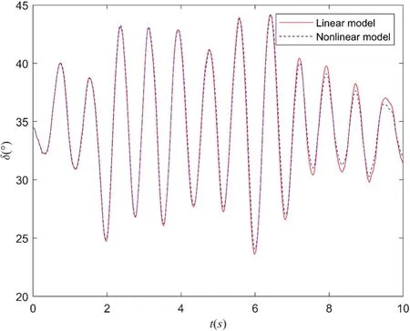
Fig.2 Comparison of power angle curves between linear and nonlinear models of the system (σ=0.234)

As seen in Fig.2, the maximum error of the power angle of the linear and nonlinear stochastic dynamic models is 0.99484°, within the constraint range.In 0–7 s,the amplitude of power angle oscillation increases while in the 7–10 s range, the power angle oscillation shows attenuation and gradually tends toward being stable.

The proposed method is compared with the Euler-Maruyama numerical calculation method (as Euler-Maruyama, Milstein and other numerical methods have the same numerical discrete format, the Euler-Maruyama numerical method is thus used as an example for comparative analysis).The Euler-Maruyama method is used for numerical discretization, and the optimal threshold model of the stochastic excitation intensity of power systems is solved.σc=0.198 is obtained in the same constraint range, and the simulation results of the power angles are shown in Fig.3 (In the simulation results, EM represents the Euler-Maruyama numerical calculation method).

In Fig.3,the curves fluctuate up and down periodically around the initial value and the error is within the constraint range.The fluctuation trend of each time period is the same as Fig.2, which indicates that the Milstein-Euler predictor-corrector method proposed in this paper is effective.

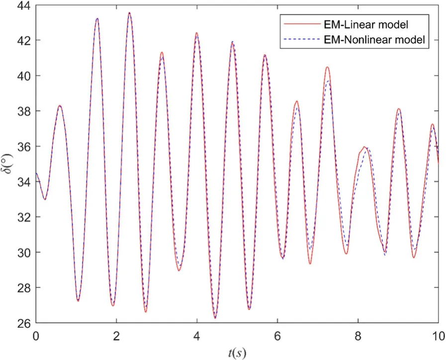
Fig.3 Comparison of power angle curves between linear and nonlinear models of the system (σ=0.198)

Comparing the threshold range of different algorithms,if the algorithm allows the model to be linearized effectively in a wider excitation range, then the algorithm has stronger adaptability.The simulation results show that the threshold range obtained by the Milstein-Euler predictor-corrector method is wider than that obtained by the Euler-Maruyama method.The Euler-Maruyama method cannot linearize the stochastic dynamic model when the excitation intensity is greater than 0.198, while the Milstein-Euler predictor-corrector method becomes unable to linearize the stochastic dynamic model only when the excitation intensity is greater than 0.234.Therefore, the proposed Milstein-Euler predictorcorrector method is more adaptable than the Euler-Maruyama and other numerical calculation methods.

After obtaining the excitation intensity threshold σc, a simulation analysis is performed using the linear and nonlinear stochastic dynamic models depending on the relative values of stochastic excitation intensities and the threshold.The power angle curves between the linear and nonlinear stochastic dynamic models are compared,and the influence of different stochastic excitation intensities on power system stability is analyzed to verify the correctness and rationality of the proposed method.

6.2 Stability analysis of stochastic excitation intensities less than the threshold value

With the stochastic excitation intensity σ ≤σc, the simulation analysis is carried out on stochastic excitation intensities of 0.05, 0.1, 0.15 and 0.20, and the simulation results are shown in Figs.4, 5, 6 and 7 respectively.The maximum error and simulation efficiency of the power angle curves corresponding to the linear and nonlinear stochastic dynamic models are shown in Table 2.(The percentage efficiency improvement is of the simulation efficiency of the linear relative to the nonlinear model).

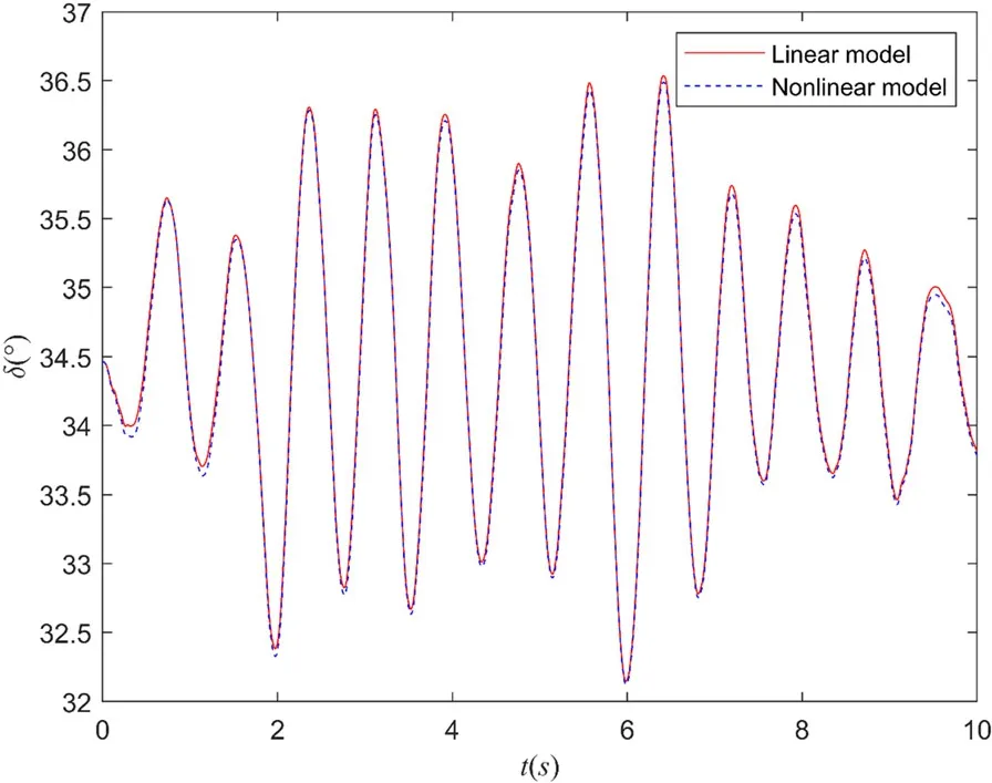
Fig.4 Comparison of power angle curves between linear and nonlinear models of the system(σ=0.05)

Fig.5 Comparison of power angle curves between linear and nonlinear models of the system (σ=0.1)

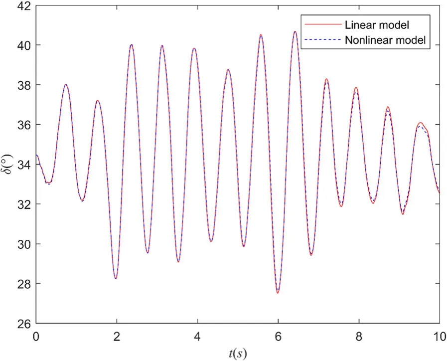
Fig.6 Comparison of power angle curves between linear and nonlinear models of the system (σ=0.15)

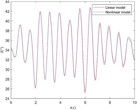
Fig.7 Comparison of power angle curves between linear and nonlinear models of the system (σ=0.2)

As seen in Figs.4, 5, 6 and 7 and Table 2, for σ ≤σc,the power angle curves of the linear and nonlinear stochastic dynamic models of the system only have small errors.With the increase of the stochastic excitation intensity, the maximum error of the power angle curves gradually increases.Within the controllable error range,the power angle curves coincide and the stability conclusions obtained are the same.Therefore,when the threshold condition is met, it is effective to convert the nonlinear model to a linear model using the predictorcorrector method.It will only bring bounded stochastic fluctuations without creating new stability problems.With the linear stochastic dynamic model, the simulation efficiency is significantly improved compared to the nonlinear one as shown in Table 2.

Table.2 Power angle error and simulation efficiency when excitation intensity is less than threshold

6.3 Stability analysis of stochastic excitation intensities greater than the threshold value

To verify the influence of linearization on the system when the stochastic excitation intensity σ>σc, stochastic excitation intensities of 0.3, 0.6 and 0.8, which are greater than the threshold, are selected for simulation analysis.The simulation results are shown in Figs.8, 9 and 10.

In Figs.8 and 9, the power angle curves of the linear and nonlinear stochastic dynamic models of the system have similar trends, although the errors become nonnegligible.In Fig.10, for the linear model, the overall power angle curve shows a stable trend, while for the nonlinear model, the system gradually becomes unstable.Under the above stochastic excitation intensities, the maximum errors of the corresponding power angle curves of the linear and nonlinear stochastic dynamic models are shown in Table 3.

Table 3 Power angle error when excitation intensity is greater than threshold

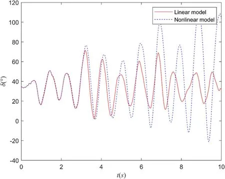
Fig.10 Comparison of power angle curves between linear and nonlinear models of the system (σ=0.8)

As can be seen, for σ>σc, the errors of the power angle curves between the linear and nonlinear models become more significant.The higher the intensity of the stochastic excitation is, the larger the maximum angle error will be.Under severe conditions, e.g., when σ=0.8,the nonlinear stochastic dynamic model becomes unstable while the linear stochastic dynamic model still shows a stable trend.Thus, the nonlinear stochastic dynamic model cannot be linearized and only the nonlinear model can be used to further analyze the stability of the power system under the stochastic excitation.

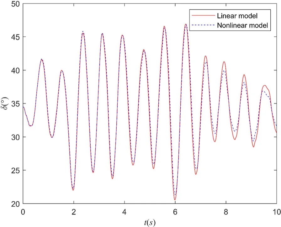
Fig.8 Comparison of power angle curves between linear and nonlinear models of the system (σ=0.3)

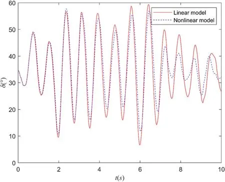
Fig.9 Comparison of power angle curves between linear and nonlinear models of the system (σ=0.6)

In summary, with the increase of stochastic excitation intensity, the errors of the power angle curves of the linear and nonlinear models increase accordingly.When the stochastic excitation intensity σ ≤σc, the power angle curves coincide and the stability conclusion is the same.Therefore, the nonlinear stochastic dynamic model can be linearized to further analyze the stability of a power system under stochastic excitation, so as to improve the efficiency of calculation and simulation.Conversely, for σ>σc, the errors of the power angle curves of the linear and nonlinear stochastic dynamic models of the system become significant.In this case, the nonlinear stochastic dynamic model cannot be linearized but it needs to be used for further analysis.Thus, determining the stochastic excitation intensity threshold is the premise to obtain a power system model and stability under the influence of reliable and effective stochastic excitation.

7 Conclusions

In this paper, the Milstein-Euler predictor-corrector method for the stochastic dynamic model of power system is constructed, the threshold discrimination basis for linearizing the nonlinear stochastic dynamic model is proposed, and the influence of different stochastic excitation intensities on the stability of the system is quantitatively analyzed.The simulation analysis shows that: 1) When the stochastic excitation intensity σ ≤σc, the errors of the linear and nonlinear stochastic dynamic models of the system can be neglected, and the stability conclusions obtained by using the two models are consistent.Thus, the nonlinear stochastic dynamic model can be linearized and the linear model can be used to analyze the system stability so as to improve simulation efficiency.When the stochastic excitation intensity σ>σc, the errors of the linear and nonlinear stochastic dynamic models of the system become non-negligible and the stability conclusions obtained diverge.Thus, it is necessary to use the nonlinear stochastic dynamic model to analyze the stability of the system.2) When the Gaussian stochastic excitation intensity is less than the threshold, it will only bring bounded stochastic fluctuations to the power system without generating new stability problems.However, when the stochastic excitation intensity is greater than the threshold, the operating state will deviate from its stable equilibrium point, and therefore, the stability of the system needs to be further examined.

The emphases and difficulties of further research are as follows: 1) How to effectively evaluate explicit stochastic excitation intensity; 2) How to construct the stochastic dynamic model and algorithm to analyze the stability of the power system under the interference of multiple noises and multiple types of stochastic excitation.3) How to apply the proposed method to multimachine power systems.

Acknowledgements

This work was supported by the National Natural Science Foundation of China (52077189) and Natural Science Foundation of Hunan Province(2020JJ4577).The authors also sincerely thank the organizations and individuals, whose work has been cited in this article.

Authors’ contributions

L.L., Y.C.and H.L.conceived the idea.L.L., Y.C.and H.L.participated in the design of the study and performed the analysis.L.L., Y.C., H.L., B.Z.and Y.L.conceived of the study, and participated in its design and coordination.L.L.,Y.C., H.L., B.Z.and Y.L.helped to draft the manuscript.All authors wrote the manuscript.All authors read and approved the final manuscript.

Funding

This work was supported by the National Natural Science Foundation of China (52077189) and Natural Science Foundation of Hunan Province(2020JJ4577).

Availability of data and materials

Data sharing not applicable to this article as no datasets were generated or analyzed during the current study.

Declarations

Ethics approval

This article does not contain any studies with human or animal subjects performed by author.

Competing interests

The authors declare that they have no competing interests.