Generating Adversarial Samples on Multivariate Time Series using Variational Autoencoders
Samuel Harford,, Fazle Karim, and Houshang Darabi,
Abstract—Classification models for multivariate time series have drawn the interest of many researchers to the field with the objective of developing accurate and efficient models. However,limited research has been conducted on generating adversarial samples for multivariate time series classification models.Adversarial samples could become a security concern in systems with complex sets of sensors. This study proposes extending the existing gradient adversarial transformation network (GATN) in combination with adversarial autoencoders to attack multivariate time series classification models. The proposed model attacks classification models by utilizing a distilled model to imitate the output of the multivariate time series classification model. In addition, the adversarial generator function is replaced with a variational autoencoder to enhance the adversarial samples. The developed methodology is tested on two multivariate time series classification models: 1-nearest neighbor dynamic time warping(1-NN DTW) and a fully convolutional network (FCN). This study utilizes 30 multivariate time series benchmarks provided by the University of East Anglia (UEA) and University of California Riverside (UCR). The use of adversarial autoencoders shows an increase in the fraction of successful adversaries generated on multivariate time series. To the best of our knowledge, this is the first study to explore adversarial attacks on multivariate time series. Additionally, we recommend future research utilizing the generated latent space from the variational autoencoders.
I. INTRODUCTION
MACHINE learning drives many facets of society including online search engines, content analysis on social networks, and smart appliances such as thermostats. In computer vision, machine learning is commonly used for recognizing objects in images or video [1], [2]. In natural language processing for transcribing speech into text, matching news articles, and selecting relevant results [3], [4]. In healthcare, to diagnose and predict patient’s survival [5], [6].
Time series classification is a subfield of machine learning that has received a lot of attention over the past several decades [7], [8]. A time series can be univariate or multivariate. Univariate time series are a time ordered collection of measurements from a single source. Multivariate time series are time ordered collections of measurements from at least two sources [9]. While most time series research focused on univariate time series [10]–[17], research in the area of multivariate time series has increased over the past decade [18]–[21]. Multivariate time series classification is applied in fields including healthcare [22], manufacturing[23], and action recognition [24]. Time series classification models aim to capture the underlying patterns of the training data and generalize the findings to classify unseen testing data. The field of multivariate time series classification has primarily focused on more traditional algorithms, including 1-nearest neighbor dynamic time warping (1-NN DTW) [25],WEASEL+MUSE [19], and Hidden-Unit Logistic Model [18].With the surge in computational power, deep neural networks(DNNs) are increasingly being applied in machine learning applications [26], [27]. Due to their simplicity and effectiveness, DNN are becoming excellent methods for time series classification [20], [28], [29].
While machine learning and deep learning techniques allow for many important and practical problems to be automated,many of the classifiers have proven to be vulnerable to adversarial attacks [30], [31]. An adversarial example is a sample of input data that has been slightly modified in a way that makes the classifier mislabel the input sample. Similar examples can be created by generative adversarial networks(GANs), which look to generate data instances similar to that of the modeling data but not aim to manipulate classifiers[32]–[34]. In the field of computer vision, it has been shown that image recognition models can be tricked by adding information to an image that is not noticeable to the human eye [31]. Although DNNs are powerful models for a number of classification tasks, they have proven to be vulnerable to adversarial attacks when minor carefully crafted noise is added to an input [35], [36]. These vulnerabilities have a harmful impact on real-world applicability where classification models are incorporated in the pipeline of a decision making process [37]. A significant amount of research in adversarial attacks has focused on computer vision. Papernotet al.’s work has shown that it is easy to transfer adversarial attacks on a particular classifier to other similar classifiers [38]. Recent years have shown an increased focus on adversarial attacks in the field of time series classification [39]–[42]. However, these studies have been limited to attacks on univariate time series.
Many strategies have been developed for the generation of adversarial samples to trick DNN models. Most techniques work by targeting the gradient information of DNN classifiers[43]–[45]. In time series classification, classifiers used to monitor the electrocardiogram (ECG) signals of a patient can be manipulated to misclassify important changes in a patient’s status. When attacking traditional time series classifiers, it is important to note that the model mechanics are nondifferentiable. For this reason, attacks are not able to directly utilize the gradient information from traditional models. There are two main types of attacks. Black-box (BB) attacks rely only on the models output information, the training process and architecture of the target models. White-box (WB) attacks gives the attacker all information about the attacked model,including the training data set, the training algorithm, the model’s parameters and weights, and the model architecture[45].
This study proposes extending the gradient adversarial transformation network (GATN) methodology to attack multivariate time series and utilize different adversarial generators [40]. GATN is extended by exploring the use of adversarial autoencoders to generate adversarial samples under both black-box and white-box attacks. The GATN methodology works by training a student model with the objective of replicating the output behavior of a targeted multivariate time series classifier. The targeted model is referred to as a teacher model. Once the student model has learned to mimic the behavior of the teacher model, the GATN model can learn to attack the student model. This study uses the 1-NN DTW and fully convolutional network(FCN) as the teacher models. Given a trained student model,the proposed multivariate gradient adversarial transformation network (MGATN) is then trained to attack the student model.Our methodologies are applied to 30 multivariate time series bench marks from the University of East Anglia (UEA) and the University of California, Riverside (UCR) [46]. To the best of our knowledge, this is the first study to conduct adversarial attacks on multivariate time series.
The remainder of this paper is structured as follows: Section II provides a background on the utilized multivariate time series classification models and techniques for creating adversaries.Section III details our proposed methodologies. Section IV presents the experiments conducted on the benchmark multivariate time series models. Section V illustrates and discusses the results of the experiments. Section VI concludes the paper and proposes future work.
II. DEFINITIONS AND BACKGROUND
For the task of multivariate time series classification, each instance is a set of time series which may be of varying lengths.
Definition 1:Univariate Time SeriesT=t1;t2;...;tnis a time ordered set of lengthncontinuous values. The length of a time series is equal to the number of values. A time series dataset is a collection of time series instances.
This work focuses on multivariate time series.
Definition 2:Multivariate Time Series consist ofMunivariate time series, where theMis the number of dimensions andM≥2

Each multivariate time series instance has a corresponding class label. The objective of multivariate time series classification is to develop models that can accurately identify the class label of an unseen instance.
A. Multivariate Time Series Classifiers

whereirefers to the position on time seriesQandjrefers to the position on time seriesC. The warping matrix is initialized as

2) Multi Fully Convolutional Network
Inspired by their success in the fields of computer vision and natural language processing, deep learning models have been successfully applied to the task of time series classification [20], [28], [52]. The multivariate fully convolutional network (Multi-FCN) is one of the first deep learning networks used for the task of multivariate time series classification. Fig. 1 illustrates the Multi-FCN network. The three convolutional layers output filters of 128, 256, and 128 with kernels sizes of 8, 5, and 3, respectively. The model outputs a class probability for use in class labeling.

Fig. 1. The Multi-FCN architecture.
B. Adversarial Transformation Network
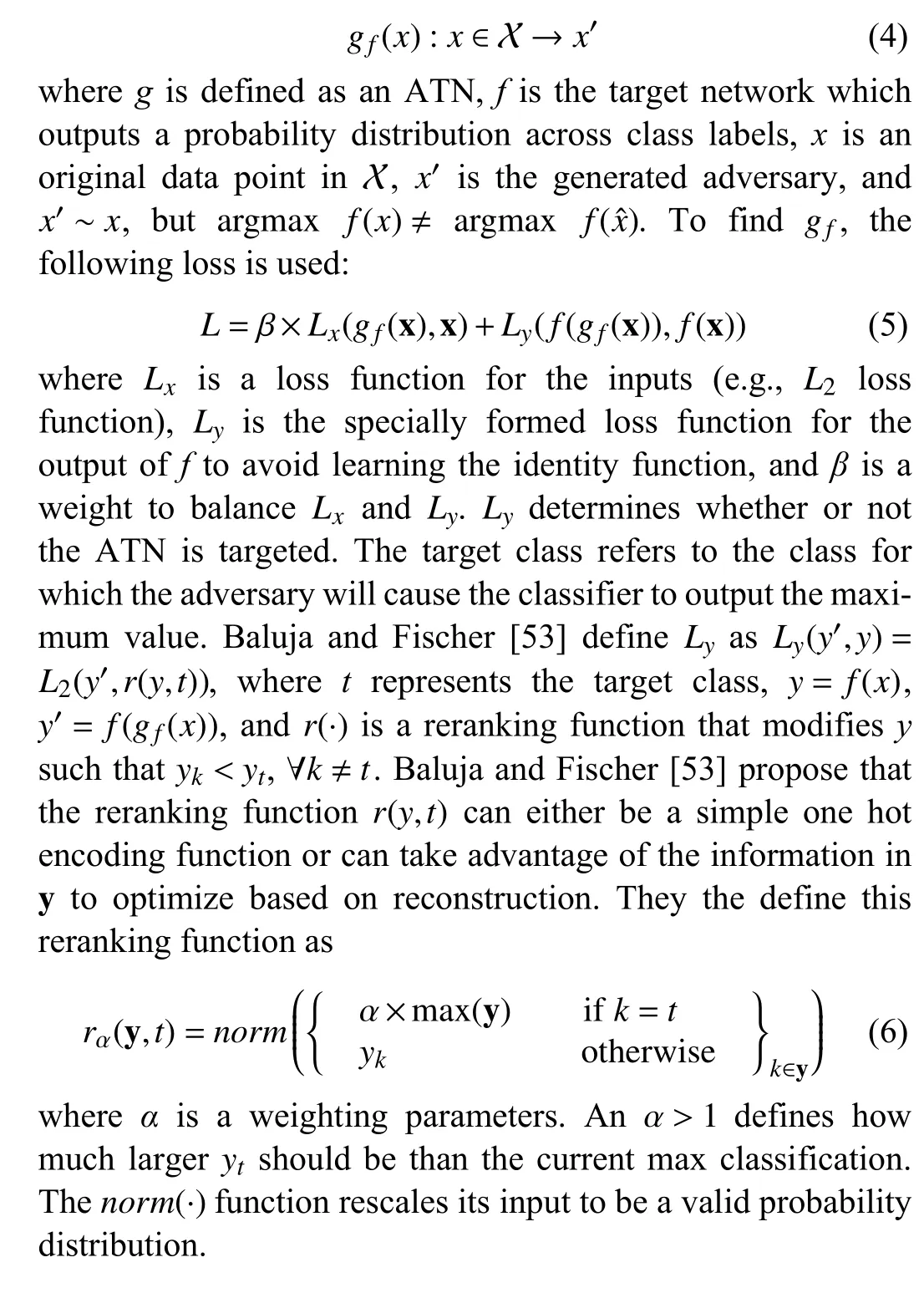
Multiple approaches for generating adversarial samples have been proposed to attack classification models. These methods have focused on classification tasks in the field of computer vision. Most methods use the gradient information with respect to the input sample or directly solving an optimization problem on the input sample. Baluja and Fischer[53] introduce adversarial transformation network (ATN), a neural network that transforms an input into an adversarial example by using a target network. ATNs may be trained for black-box or white-box attacks. ATNs work by first using a self-supervised method to train a feed-forward neural network.The model works by taking an original input sample and making slight modifications to the classifier output with the objective of matching the adversarial target. An ATN is defined as a neural network
C. Transferability Property
The transferability property of an adversarial sample is the property that the same adversary produced to mislead a targeted modelfcan mislead another models, regardless of model architecture [54], [55]. Papernotet al.[38] further study this property and propose a black-box attack by training a local substitute network,s, to replicate the target model,f.The local substitute networksis trained using generated samples and the targeted modelfis used to get the output label of generated samples. The transferability property is utilized in adversarial attacks by exploiting the full local modelson the targeted modelfwith the objective of achieving misclassifications. Papernotet al.[38] show that this method can be applied on both DNN and traditional machine learning classifiers.
D. Knowledge Distillation
A key strategy for reducing the cost of inference is model compression, also known as knowledge distillation [56]. The idea of knowledge distillation is to replace the original,computationally expensive model with a smaller model that requires less memory, parameters and computational time.This idea works by training a smaller student modelsto mimic the behavior of the larger teacher modelf. The teacher modelfhas its knowledge distilled into the student modelsby minimizing a loss function between the set of networks. This loss function aims to output the same class probability vector on the student modelsas that generated by the teacher modelf. Hintonet al. [57] state that the commonly used softmax function results in a skewed probability distribution where the correct probability class is very close to 1 and the remaining classes are close to 0. To reduce the resulting skewness in the probability class vector, Hintonet al. [57] recommends adjusting the output such that

E. Gradient Adversarial Transformation Network


F. Adversarial Autoencoders
Makhzaniet al. [58] propose the adversarial autoencoder(AAE), which is a probabilistic autoencoder that utilizes the knowledge learned from generative adversarial networks(GANs) [59]. The GANs are used to perform variational inference by matching the aggregated posterior of the hidden code vector of the autoencoder with an arbitrary prior distribution. AAE are similar to standard autoencoders [60],where the objective is to accurately reconstruct the original input, subject to a limited amount of added noise.
In addition to simple autoencoders, Makhzaniet al. [58]propose the use of variational autoencoders (VAE) [61].VAEs provide a formulation in which the encodingzis interpreted as a latent variable in a probabilistic generative model, a probabilistic decoder is defined by a likelihood functionpθ(x|z) and parameterized byθ. Alongside a prior distributionp(z) over the latent variables, the posterior distributionpθ(z|x)∝p(z)pθ(x|z) can then be interpreted as a probabilistic encoder. Fig. 2 illustrates this process. Ideally,the trained latent vector creates clusters that are as close as possible to each other while still being distinct, allowing smooth interpolation, and enabling the construction of new samples. To better create the latent vector a Kullback-Leibler(KL) divergence is introduced into the loss function [62]. The KL divergence between two probability distributions simply measures how much they diverge from each other.Minimizing the KL divergence here means optimizing the probability distribution parameters to closely resemble that of the target distribution. The KL divergence defined as

Fig. 2. The VAE architecture.

wherenis the length of the output,Pis the probabilistic distribution of the original data, andQis the probabilistic distribution of the adversarial data. Due to the limited information about the actual probabilistic distributions,Variational Inference is used to simplify the divergence calculation using known information [63]. The KL diverence is simplified to

whereμis the mean output of the encoding layer, andσis the standard deviation output of the encoding layer.
III. PROPOSED METHODOLOGY
A. Multivariate Gradient Adversarial Transformation Network
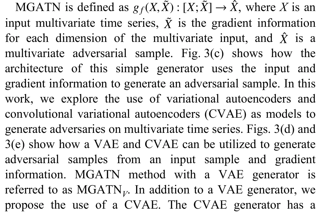
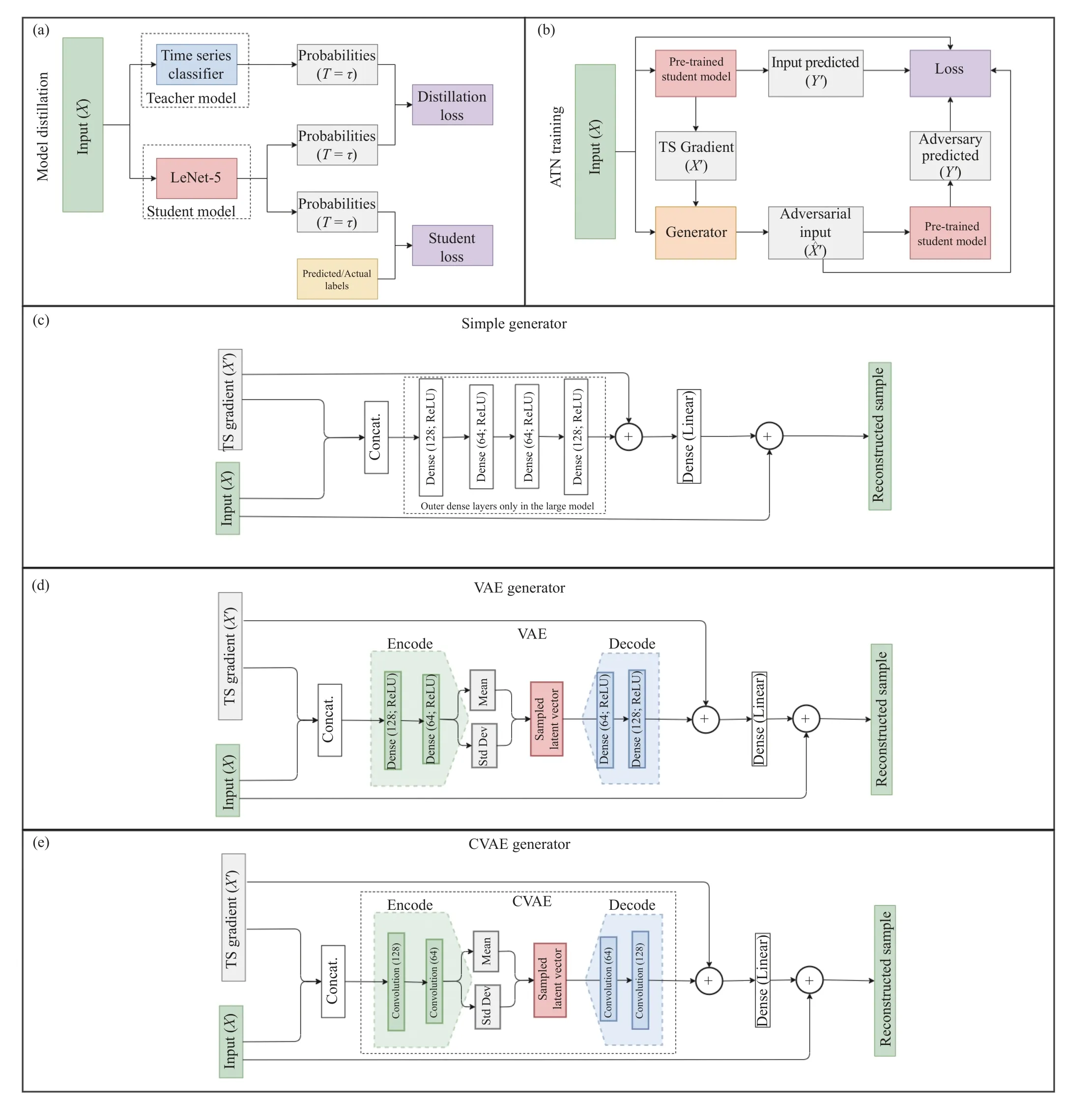
Fig. 3. The subfigures (a) and (b) illustrate the methodology of training the model distillation used the attacks. The subfigures (c) and (d) illustrate the methodology utilized to attack a time series classifier.
The use of the GATN has proven to be a successful method for developing adversarial samples on univariate time series[40]. However, GATN and other adversarial attacks on time series have not been applied on multivariate time series. In this work, we purpose multivariate gradient adversarial transformation network (MGATN) which extends the GATN model for use in generating multivariate adversarial time series. In addition, we explore the use of Variational Encoders and Convolution Variational Encoders as alternative generator functions.similar architecture to the VAE generator, where the dens e layers of the encoder and decoder are modified to 1-D convolutional layers. MGATN method with a CVAE generator is referred to as MGATNCV. The MGATNCVgenerator encodes the samples by first passing through an intermediate convolutional layer of filter size 32 and kernel size 5, then feeds to two branched convolutional layers of filter size 16 and kernel size 5. The two convolutional layers then pass through a sampling layer. The final step decodes the sampling layer with two convolutional layers of filter size 32 and the original time series shape, both with kernel sizes or 5.
B. Training Methodology
This subsection discusses the training purpose for the MGATN methodology. Figs. 3(a) and 3(b) illustrates the full framework architecture defined in [15]. The framework architecture is similar to that of GATN, with notable modifications. The input to the framework is multivariate,where the shape of inputs changes from (batch size, length,value) to (batch size, channel, length, value). This increase in shape requires the student model to be modified to a LeNet-5 with 2D Conv layers. In addition, we explore different generator functions to create adversarial samples. The tested generator functions include a fully connected network, a variational autoencoder, and a convolutional variational autoencoder. Figs. 3(c)–3(e) illustrate the generator architectures. Fig. 3(c) illustrates the simple generator where the MGATN uses two dense layers in the autoencoder block. For a fair comparison of model parameters, a MGATNLis included in the experiments and results. MGATNLand MGATNVhave about the same amount of parameters as they have the same number and size of dense layers. Figs. 3(d) and 3(e) illustrate both the VAE and CVAE generators where the VAE utilizes dense layers in the encoder/decoder blocks and CVAE utilize convolutional layers in the encoder/decoder blocks.
The loss calculation is dependent upon the choice the the reranking function, as discussed in Section II-B. The simplest form of the reranking function is a one hot encoding of the desired class label. However, the one hot encoding reranking fuction is not the best choice when the objective is to minimize perturbations per class label. Other options for reranking functions require the use of the class probability vector. This class probability vector is not available when performing black-box attacks or when attacking most traditional models. We utilize the transferability property and knowledge distillation to train a student networks, where the class probability vector is not available. The student neural networksis trained to mimic the classification output for the targeted modelf. The student model of the proposed architectures (MGATN, MGATNL, MGATNV, and MGATNCV) uses the same knowledge distillation loss function described in Section II-E. The knowledge learned from the student model is then used in substitute of the unknown information, such as the class probability vector.
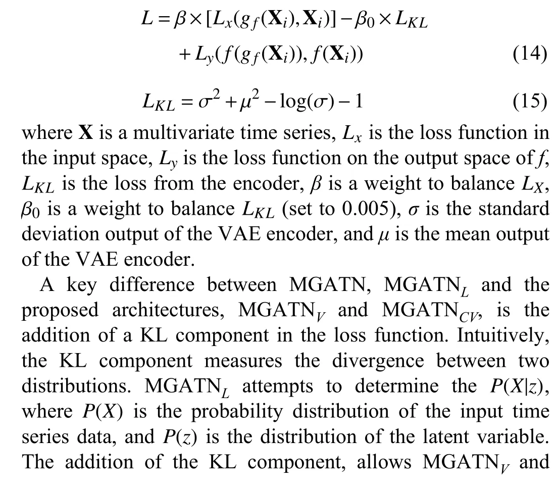
The MGATN framework aims to optimize the adversarial samples by balancing the loss on the input space and the loss of the prediction output. This loss function is described in (5).When training with VAE and CVAE generators, the KL divergence must be factored into the loss equation. The following loss function is optimized:
IV. EXPERIMENTS
A. Multivariate Time Series Benchmarks
All methodologies presented in this work are tested on 30 multivariate time series benchmark datasets. These benchmarks are compiled and provided by University of East Anglia (UEA) and the University of California, Riverside(UCR) in the Multivariate Time Series Classification Archive[46]. Table I provides information about the test benchmarks.These benchmark datasets are from a variety of fields,including medical care, speech recognition and motion recognition.
B. Black-Box and White-Box Restrictions
The experiments to evaluate all versions of MGATN follow specific restrictions for black-box and white-box attacks. All versions of MGATN require the use of gradient information to attack the target classifier. In this study, black-box attacks are limited to the discrete class label of the model output, and not the class probability vector that is output from a neural network with a softmax output.
C. Experimental Setup
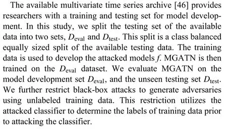
This work explores black-box and white-box attacks with different generators on traditional and neural network time series classifiers. We compare the different generator functions to present how the proposed generator functions perform in comparison to established generator functions.Details for these classifiers were explained in Section II-A.Based on the restrictions of the attacks and traditional time series classifiers, we utilize a student model for all attacksexcept the white-box attack on the Multi-FCN classifier.White-box attacks on traditional classifiers, such as 1-NN DTW, do not provide the required class probability information for MGATN to be utilized. Additionally, black-box attacks for both traditional and neural network do not allow the attacker access to the internal information of the classifier,such as the neural network weights. In these cases, the student modelsis utilized to train MGATN. The output of MGATN is then used to test if the teacher modelfis vulnerable to the adversarial sample. As discussed in Section IV-B, the initial testing set is split into two equally sized sets for evaluation,DevalandDtest. When evaluating the different variations of MGATN, we compute the fraction of successful adversaries on the targeted modelfgenerated on the evaluation setDeval.For a multivariate time series to be a successful adversarial example, we first input the time series into the classification model to see if the classifier results in the correct class label.If the classifier is able to correctly determine the class label of the time series, then we check to see if the corresponding adversarial sample of this time series is incorrectly labeled by the targeted classifier. This definition ensures that only correctly labeled samples can result in a possible adversarial sample. To evaluate our models ability to attack multivariate time series classification algorithms, we utilize both a traditional distance based classifier and a neural network classifier. The attacked time series classifiers are the Multivariate 1-Nearest Neighbor Dynamic Time Warping and the Multivariate Fully Convolutional Network. We evaluate based on the number of adversarial samples generated and the amount of perturbation added. The perturbation is measured by comparing the mean squared error of the original input sample compared to the output adversarial sample. The objective is to minimize the amount of perturbation and maximize the fraction of the training samples that result in successful adversaries. All experiments use a reranking weightαthat is set to 1.5. The target class is specified to class 0. For benchmarks that have non-numeric class labels, the labels are encoded and the corresponding class label can be found in our
codebase. The reconstruction weight parameterβis selected by grid searching over a set of possibilities, such that β ∈{0.1,0.05,0.01,0.005,0.001,0.0005,0.0001,0.00001}. This work performs several experiments to show how multivariate time series classifiers can be attacked (comparing fraction of successful adversaries in Section V-A), how well the proposed architectures can generalize onto unseen multivariate time series data (generalization in Section V-B) and how well can these attacks be defended by retraining on these adversaries(defense in Section V-C).
护理前两组血糖餐前餐后监测状况、酸中毒症状积分、生存质量接近(P>0.05);护理后综合护理干预组血糖餐前餐后监测状况、酸中毒症状积分、生存质量的改善幅度更大(P<0.05)。见表 2。

TABLE I DATASET DESCRIPTION FOR UEA AND UCR MULTIVARIATE TIME SERIES BENCHMARKS
D. Modeling Parameters
All tested attacks utilize a student network to mimic the target network except white-box attacks that target the Multi-FCN classifier. ATNs can directly utilize the gradient information of the Multi-FCN model that is available to the attacker in the white-box case. White-box attacks on Multi-FCNs are evaluated directly on the target classification model.
All student models utilize a simple LeNet-5 architecture that is modified for a multivariate input [65]. The LeNet-5 architecture is selected because it is one of the earliest and simplest convolutional neural networks, which has shown to work effectively on attacking univariate time series classifiers[40]. The architecture is a convolution neural network with two 2-dimensional convolutional layers with filter of size 6 and 16, kernels of size 5 and 5, ReLU activation functions,and valid padding. Each convolutional layer is passed to a 2-D Max Pooling layer. This is then passed to a flattening layer.The network then has two dense layers of 120 and 84 with tanh activation functions. Finally the network ends with a dense softmax layer consisting of the desired number of classes.
We use the multivariate version of 1-NN DTW to evaluate adversarial attacks on traditional time series classifiers. While this classifier has proven to be an effective method for both univariate and multivariate time series, the distance based restriction requires some modifications to utilize probabilistic outputs. This is not an issue when conducting black-box attacks on the classifier. White-box attacks have access to the output class probability distribution for each sample. Karimet al. [40] introduced a method of generating a class probability distribution that can generate the same discrete class result as the original classification. This method can be extended to accept a set of distance matrices as inputs, as opposed to a single distance matrix.
Our experiments evaluate the use of four different methods networks for adversary generation. The first is a simple fully connected network, which passes the original and gradient information to two dense layers with ReLU activation functions and the output is a gradient with matching input shape and a linear activation function. The second is an extended simple generator with two additional dense layers.The third network is a variational autoencoder with an intermediate dimension of 32 and latent dimension of 16. The final network is a convolutional variational autoencoder which alters the original dense layers of the VAE with convolutional layers. This network has the same intermediate dimension of 32 and latent dimension of 16. More detailed architecture parameters can be explored in our codebase.
V. RESULTS
A. Fraction of Successful Adversaries
Fig. 4 illustrates the fraction of successful adversaries generated during black-box and white-box attacks on the 30 tested multivariate time series benchmarks. The fraction of successful adversaries is defined as the number of adversaries captured by the attack divided by the number of possible adversaries that could be generated. As an additional requirement, we select our models based on a mean squared error (MSE) limit of 0.1 between the original and adversarial time series. This requirement is used to determine the model based on the stated range of beta valuesβ. Fig. 4 also illustrate the differences in results for the tested generators. These include MGATN, MGATNL, MGATNV, and MGATNCV. The target class for all experiments is set to class 0, where string labels are encoded and these class encoding can be found in our codebase for reproducibility. The detailed results for all experiments can be found in Appendix.
There are a total of 120 experiments for each generator function, 30 datasets on 4 different attack-target combinations.We compare these experiments across generators by evaluating the number of wins a method has across all experiments. A win is defined as one method having a greater fraction of successful adversaries than any other method,where ties are not collected. The number of wins for MGATN,MGATNL, MGATNV,and MGATNCVare 16, 10, 38, and 27,respectively. MGATNVhas the most wins across all the experiments where 27 of the 38 wins occur in black-box attacks. However, MGATNCVhas a high number of white-box wins (19 wins) compared to the other methods. When looking at the target model instead of attack, we see that MGATNVhas the most wins on Multivariate 1-NN DTW (14 wins) and has the most wins on Multi-FCN (24 wins). We postulate the AutoEncoder component of MGATNVand MGATNCVto be the reason why the performance is increasing and not the size of the network. This is because MGATNLand MGATNVhave about the same size and parameters, yet MGATNVoutperforms MGATNL, significantly. These findings demonstrate the significant improvement achieved with the modification of the generator functions. Fig. 5 illustrates adversarial samples with all attacks.

Fig. 4. Black-box and white-box attacks on FCN and 1-NN DTW classifiers that are tested on Deval. Blank bars mean that the adversarial attacks did not result in any adversaries for a specific attack and dataset.
Table III summarizes the results of MGATNVand MGATNCVcompared to the original MGATN and MGATNL.Table cells in green show a significant improvement (at a pvalue of 0.05) over the original MGATN. These results show MGATNVis superior to MGATN and MGATNLwhen applied on both tested black-box attacks. Even with approximately the same number of parameters, MGATNVstatistically outperforms MGATNLfor black-box attacks. However, MGATNVdoes not perform the original MGATN or MGATNLon whitebox attacks. This difference in adversarial results comes from the VAEs objective of regularizing the latent space.MGATNCVoutperforms MGATN and MGATNLwhen applying white-box attack on the Multi-FCN classifier. The MGATNCVperforms the best for white-box on the neural network classifier, which we postulate is because the convolutional component provides superior encoding for this attack. This indicates the importance of the AutoEncoders in the generator and the significant improvement in the resultant fraction of adversaries achieved.
In order to test the distribution of the generated adversary a Cramer test is used to compare generated adversaries with the original multivariate time series. The Cramer test is a nonparametric two sampled test of the underlying distributions between multivariate sets of data [66]. The Cramer test has a null hypothesis of the two samples belonging to the same distribution and an alternative hypothesis that they are drawn from different distributions. All generated adversaries have a p-value below 0.05. These results prove that all adversaries are drawn from the same distribution as their original multivariate time series.
B. Generalization
In this subsection we evaluate the trained MGATN models on the unseen testing data,Dtest. This evaluation is important when the situation does not allow time for model retraining.This is the case when sensor data only has the time for a forward pass through the network. This evaluation is not common when generating adversaries. However, time series applications often require real-time analysis of collected data.For this reason, it is beneficial that MGATN is able to generate adversarial samples without the need for retraining.Fig. 6 illustrates the fraction of successful adversaries for all testing sets and on all attacks. These results show a similar fraction for each type of attack. The white-box attack on the Multi-FCN classifier obtains the highest fraction of successful adversaries across most datasets. Additionally, we see that the black-box attack on Multi-FCN results in the lowest fraction of successful adversaries. The black-box limitation along with the increased complexity of neural networks compared to distance based models makes it difficult to generate adversaries on black-box attacks on Multi-FCNs. This generalization shows the potential to generate adversaries based on pretrained models. This allows for MGATN to be applied on edge devices with limited computational resources and still be able to generate successful adversaries.
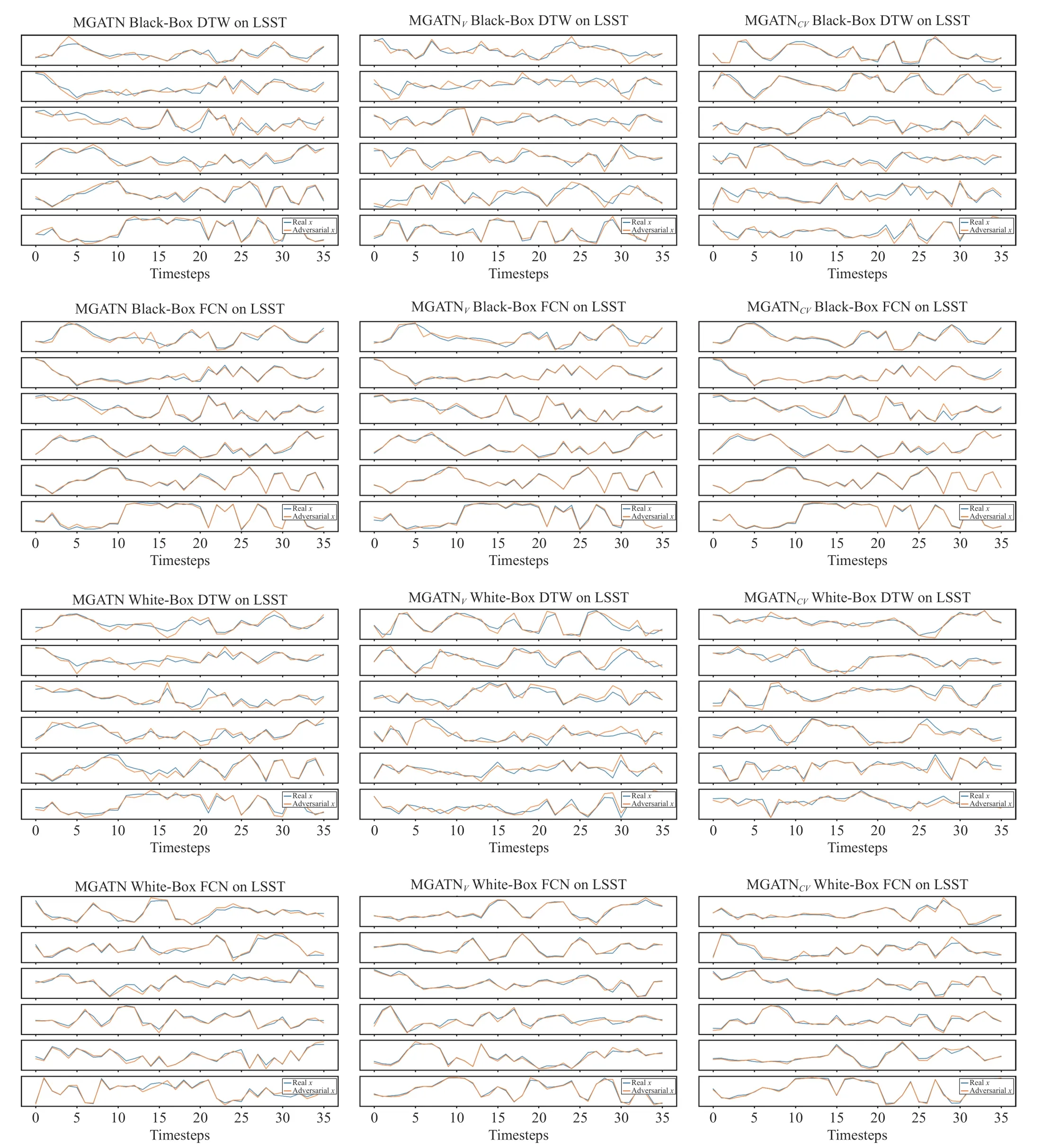
Fig. 5. Sample Adversarial Samples on the LSST dataset.
C. Defense
The ability to defend against an adversarial attack is an important post-evaluation that utilizes the findings of MGATN. In this work we explore a simple defense process that utilizes the pretrained MGATN models. Given a trained MGATN, we output the successful adversarial samples for an attack. These adversarial samples are appended onto our original training data. The classifier and MGATN are then retrained using this new training set. Based on this defense process, we evaluate MGATN by analyzing the change in testing accuracy and the fraction of successful adversaries.Table IV shows a Wilcoxon Sign-Rank Test for a comparison of testing accuracy of developed models. The testing setDtestis defined in Section IV-B. Table cells that are green show a significant improvement in testing accuracy (at a p-value of 0.05). This analysis evaluates whether the use of adversarialsample in addition to training data results in significantly higher testing accuracy. The results show that only white-box samples from Multi-FCN generated from MGATNVand MGATNCVresults in a significant increase in model accuracy.The remainder of the experiments show that the adversarial samples do not result in an improved testing accuracy when the models are retrained. Table V shows a WSRT for the comparison of the fraction of successful adversaries generated. These results show that there is a significant decrease in the fraction of adversaries generated when the model is retrained with adversaries in the training data (at a pvalue of 0.05). The one exception is the MGATNCV, where the fraction of adversaries is statistically large compared to the previous tests. This shows that both distance based and neural network classifiers become more robust when retrained with new samples.

TABLE II FRACTION OF SUCCESSFUL ADVERSARIES ON DEVAL OF OUR METHODS COMPARED TO FGSM (P-VALUE SHOWN)
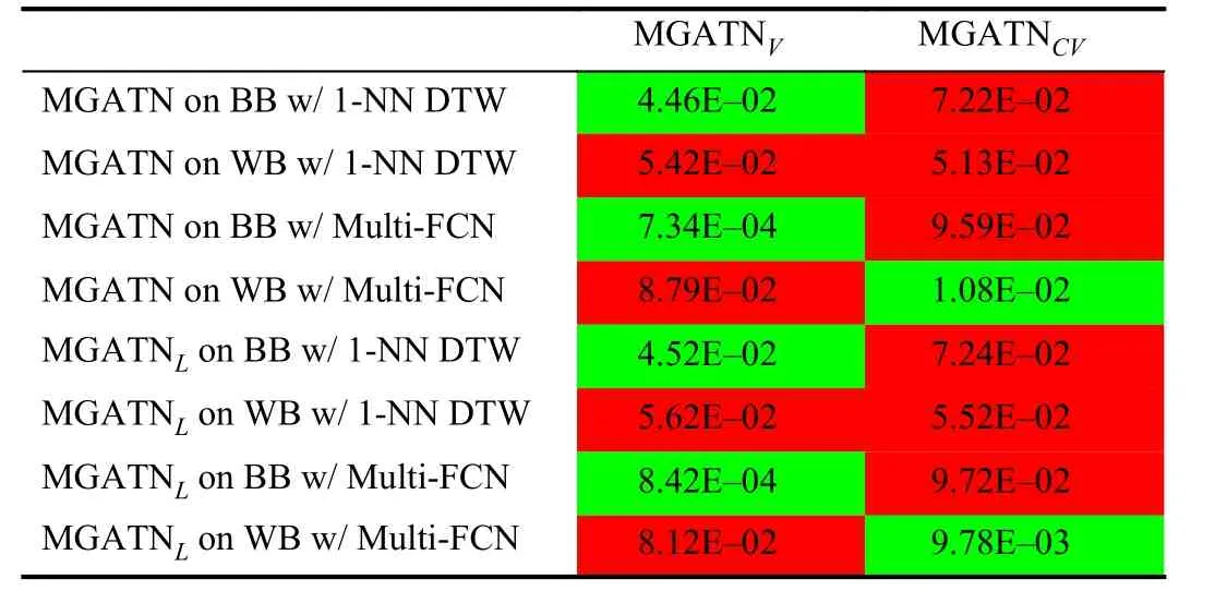
TABLE III FRACTION OF SUCCESSFUL ADVERSARIES ON DEVAL COMPARISON OF MGATN GENERATORS (P-VALUE SHOWN)
D. Latent Space
The MGATNVand MGATNCVmethods make use of variational autoencoders to generate adversarial samples.Variational autoencoders provides a probabilistic manner for describing an observation in latent space. VAEs formulate the encoder to describe a probability distribution for each latent attribute. To understand the implications of a variational autoencoder, we visualize the latent space. Fig. 7 illustrates the latent space of evaluation samples on the CharacterTrajectories dataset generated by MGATNVand MGATNCVusing a t-distributed stochastic neighbor embedding (TSNE) data reduction. TSNE is a statistical method for visualizing high-dimensional data in a two or three dimensional space using a stochastic neighbor embedding[67]. This figure shows that MGATNCVmethod is able to learn clear differences between classes. The MGATNVmethod results non-separable latent spaces using the TSNE dimensionality reduction. However, this does notmean MGATNVhas no linearly separable classes on different different or reduction techniques. Further research is required to understand the latent spaces of MGATNVModels that generate a clearly defined latent space can be used to form a generative model capable of creating new data similar to what was observed during training. New data generated from an interpretable latent space can be used to retrain classifiers to increase accuracy, further improve defense against adversarial attacks, and many other data mining applications. Further, the embeddings from the latent space can also be utilized for other classification tasks and anomaly detection.
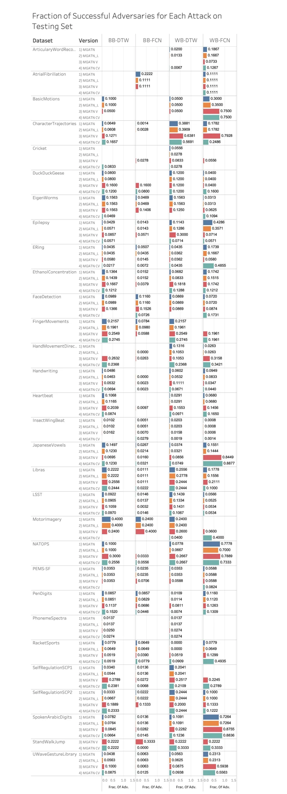
Fig. 6. Black-box and white-box attacks on FCN and 1-NN DTW classifiers that are tested on Dtest. Blank bars mean that the adversarial attacks did not result in any adversaries for a specific attack and dataset.

TABLE IV WSRT COMPARING TESTING ACCURACY OF MODELS DEVELOPED ON ORIGINALTRAINING DATA VS TRAINING DATA WITH ADVERSARIAL SAMPLES (P-VALUE SHOWN)

TABLE V WSRT COMPARING FRACTION OF SUCCESSFUL ADVERSARIES FOR MODELS DEVELOPED ON ORIGINAL TRAINING DATA VS TRAINING DATA WITH ADVERSARIAL SAMPLES (P-VALUE SHOWN)

Fig. 7. Example illustrations of Latent Dimensions using TSNE reduction.
VI. CONCLUSION
This work extends the GATN by modifying the generated function to significantly improve the generated adversaries on multivariate time series. We evaluate the different generation methods on 30 multivariate time series datasets. These evaluations test both black-box and white-box attacks on multivariate 1-NN DTW and Multi-FCN classifiers. Our results show that the most vulnerable model is the Multi-FCN attacked with white-box information. We further prove the generated adversaries are from the same distribution as the original series using a Cramer test. Utilizing an unseen testing set, we see that our MGATN models are able to generate adversaries on data without the need for retraining. A simple defense procedure shows that the use of generating adversaries when retraining our models makes them less vulnerable to future attacks while maintaining the same level of testing accuracy. Finally, we see that the latent space modeled by MGATNCVresults in a clear class separation that can be used for future data generation. Future research in this area should explore the development of targeted adversarial attacks that misclassify input to a specific class. Finally, the developed latent space information can be exploited to better understand the underlying patterns of the time series classes.
ACKNOWLEDGMENTS
We acknowledge Somshubra Majumdar for his assistance and insightful comments that laid the foundation to the research work. Further, we would like to thank all the researchers that spent their time and effort to create the data we used.
APPENDIX DETAILED RESULTS
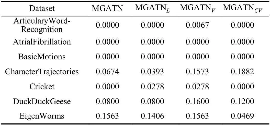
TABLE VI FRACTION OF SUCCESSFUL ADVERSARIES ON DEVAL FOR THE BLACK-BOX ATTACK ON MULTI 1-NN DTW
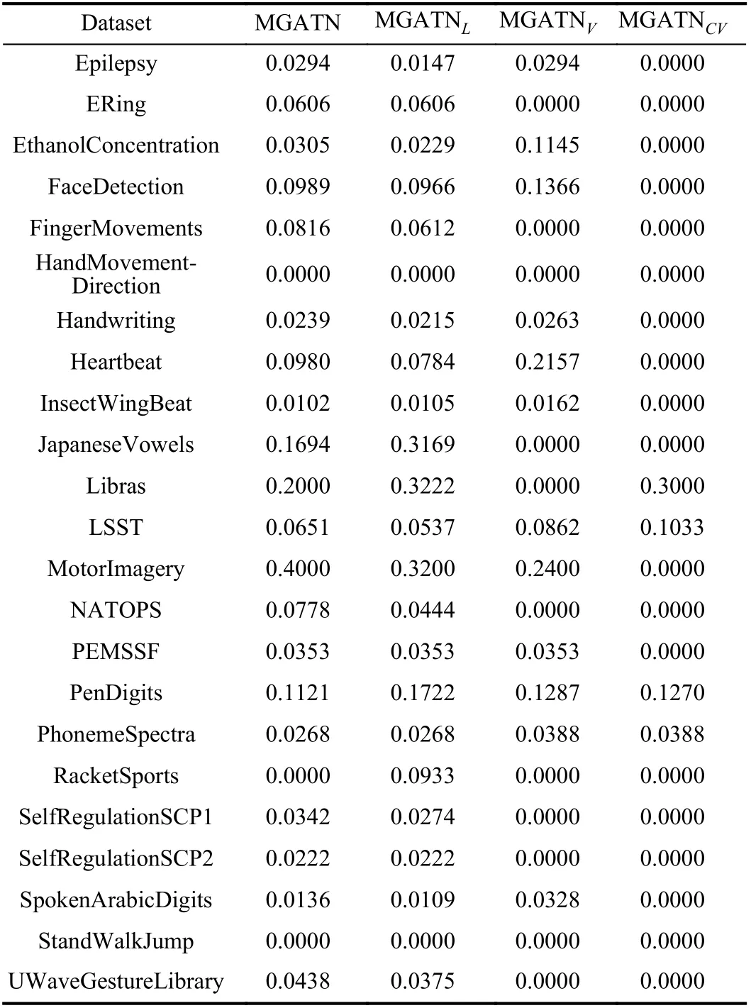
TABLE VI FRACTION OF SUCCESSFUL ADVERSARIES ON DEVAL FOR THE BLACK-BOX ATTACK ON MULTI 1-NN DTW (CONTINUED)

TABLE VII FRACTION OF SUCCESSFUL ADVERSARIES ON DEVAL FOR THE BLACK-BOX ATTACK ON MULTI-FCN
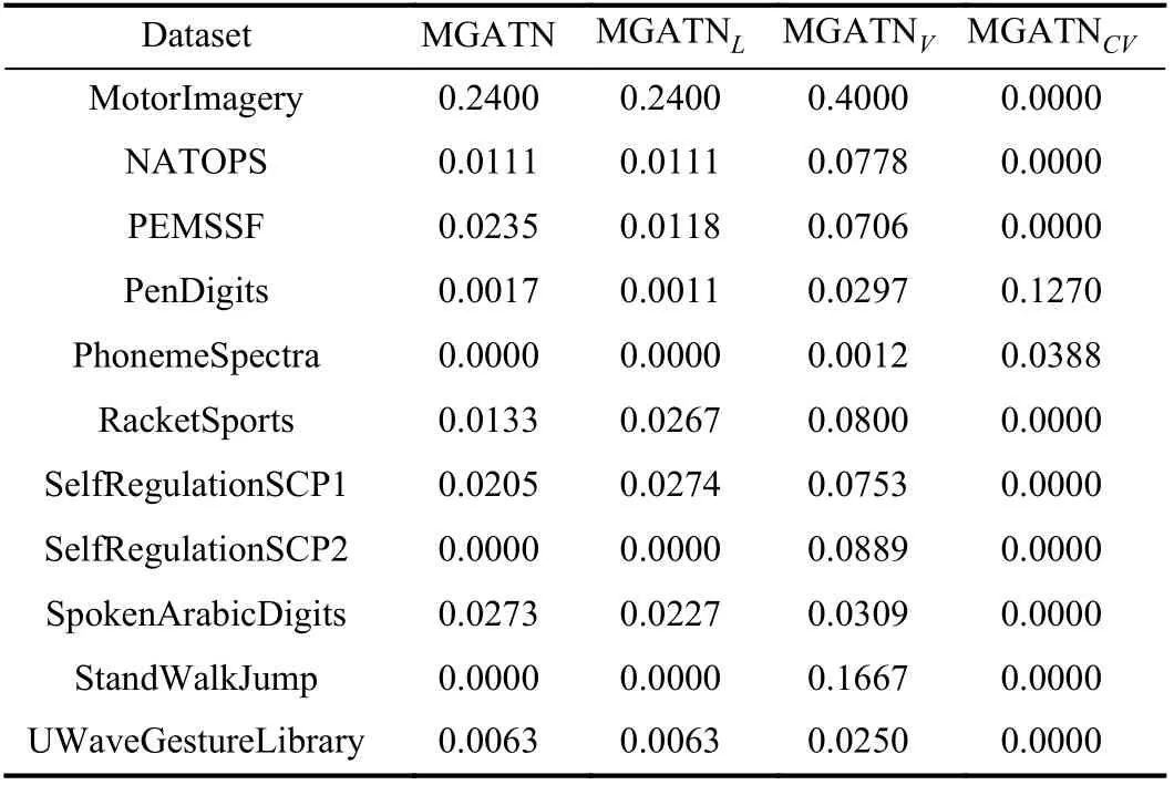
TABLE VII FRACTION OF SUCCESSFUL ADVERSARIES ON DEVAL FOR THE BLACK-BOX ATTACK ON MULTI-FCN (CONTINUED)

TABLE VIII FRACTION OF SUCCESSFUL ADVERSARIES ON DEVAL FOR THE WHITE-BOX ATTACK ON MULTI 1-NN DTW

TABLE IX FRACTION OF SUCCESSFUL ADVERSARIES ON DEVAL FOR THE WHITE-BOX ATTACK ON MULTI-FCN
 IEEE/CAA Journal of Automatica Sinica2021年9期
- IEEE/CAA Journal of Automatica Sinica的其它文章
- Distributed Resource Allocation via Accelerated Saddle Point Dynamics
- Fighting COVID-19 and Future Pandemics With the Internet of Things: Security and Privacy Perspectives
- Soft Robotics: Morphology and Morphology-inspired Motion Strategy
- A Unified Optimization-Based Framework to Adjust Consensus Convergence Rate and Optimize the Network Topology in Uncertain Multi-Agent Systems
- Vision Based Hand Gesture Recognition Using 3D Shape Context
- MU-GAN: Facial Attribute Editing Based on Multi-Attention Mechanism
