Threshold Dynamics of Discrete Meningococcal Meningitis Model with Vaccination and Therapy
MA Xia, CAO Hui, ZHANG Jin-zhu, GUO Zun-guang
(1- Department of Science, Taiyuan Institute of Technology, Taiyuan 030008;2- College of Science, Shaanxi University of Science and Technology, Xi’an 710021)
Abstract: According to the epidemic characteristics of Meningococcal Meningitis in China and the influence of vaccination factors, we formulate a discrete-time SCIRS model with vaccination and therapy by using the backward Euler method and investigate its dynamic characteristics. We obtain sufficient conditions for the global behavior of the equilibrium points by constructing suitable Lyapunov functions. We further conclude that the disease is permanent by using the theory of persistence in dynamical systems.Numerical simulations are carried out to illustrate the main theoretical results.
Keywords: discrete Meningococcal Meningitis model; backward Euler; persistent; globally asymptotically stability; Lyapunov function; numerical simulation
1 Introduction
Meningococcal Meningitis is an acute respiratory epidemic caused by cerebrospinal meningitis diplococcus from a variety of serums. It is transmitted primarily through airborne droplets, or directly contacting with secretion of respiratory tract or gullet from patients or healthy carriers. It doesn’t have animal or environmental host. The person carrying bacterium and infectious patient are the infection source. Meningococcal Meningitis mainly threaten the health of children and its mortality rate is still very high.
The meningococcus can asymptomatically inhabit the nasopharynx and a population of around 10%asymptomatically carry meningococcus in the nasopharynx[1]. Only a small proportion of carriers develops invasive disease, the duration of carriage can be from 1 week to 1 year[2,3]. Vaccination is considered to be a successful intervention policy as well as a cost-effective strategy to reduce both the morbidity and mortality of individuals[4]. It has been used to control epidemic diseases such as chicken pox,measles, mumps, phthisis, hepatitis B and influenza. However, vaccination does not necessarily imply life-long immunity for a vaccinated person. In some cases, vaccination is ineffective and fails to provide immunity,sometimes immunity acquired through vaccination wanes and does not provide life-long protection[5,6].
Since the current MPV(MPV is the abbreviations of Meningococcal Polysaccharide Vaccine)group A and C conjugate vaccine does not last long immunity for children and adults, and the protective effect on infants is very poor. Furthermore, it is practically impossible to vaccinate all susceptible individuals and the coverage rate is not high in remote villages. Hence, it is of great importance to determine a fraction of immune individuals in a population called the herd immunity threshold, so the local outbreak often occurs[7]. Though vaccination does not prevent carriers from carrying neisseria meningitis, it can stimulate the herd immunity that reduces the disease outbreak. The MCC (MCC is the abbreviations of Meningococcal C group of Conjugate vaccine)vaccine has been shown to significantly reduce the carriage of neisseria meningitides[8].So the vaccine factors should be considered in the model.
Several mathematical models have been proposed to study the epidemic characteristics of Meningococcal Meningitis. Maria and Crispino-O’Connell[9]constructed a Meningococcal Meningitis PDE model with age structures,studied the effect of carriers on disease. Trotteret al[3]built an epidemic model with age structures based on the immune data in England and Wales to analyze the direct and indirect effects of C conjugate vaccine. Guzzettaet al[10]considered the difference between the epidemic risk of first infection and second infection. The results showed that the incidence rate of second infection was 100 times smaller than first infection. Irvinget al[1]used a definite compartment model to explore the impact of seasonal factors in disease transmission.
Since statistical data on epidemics is announced in discrete time together with the new cases of notifiable communicable diseases. It is more convenient and accurate to describe epidemics using discrete-time models because they permit arbitrary time step units[11,12]. Motivated by the above ideas, we formulate a discrete Meningococcal Meningitis SCIRS model with vaccination and therapy by using the backward Euler scheme called ‘mixed type’ formula[13,14], and investigate the global dynamical behaviors. The discrete SCIRS model and the positivity, boundedness of the solution are presented in next section. The global stability of disease-free equilibrium point and persistence of the disease are acquired in section 3. The existence and sufficient condition for global stability of endemic equilibrium are obtained in section 4. Numerical simulations are done to illustrate and extend the main theoretical results in section 5.Discussions are presented in the last section.
2 A discrete Meningococcal Meningitis SCIRS model
According to the spread characteristics of Meningococcal Meningitis in China, we establish a discrete SCIRS model by using the backward Euler scheme (which is called mixed type formula,see[13,14])based on the reference[1]. LetN(n)denote the number of the host population,S(n),C(n),I(n) andR(n) be the numbers of individuals in the susceptible, asymptomatic carrier, infective, and recovered compartments at timen, respectively. The discrete SCIRS model is
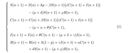
where Λ is the constant recruitment rate,pis the ineffective ratio of newborn vaccine,dis the proportion of the susceptible that is effectively vaccinated,εis the infection ratio of carriers relative to infectives,βis the transmission rate,μis the natural death rate,θis the risk of disease given infection,αis the rate of losing carriage,δis the death rate caused by disease, andγis the recovery rate.φis the rate of losing immunity. The biological background requires that all parameters are non-negative. As the epidemiological background of model(1),we assume that any solution of model(1)satisfies the following initial conditionS(0)>0, C(0)>0, I(0)>0, R(0)>0.
Theorem 1 Every solution (S(n),C(n),I(n),R(n)) of model (1) with nonnegative initial values are positive and ultimately bounded for alln >0.
Proof From the first equation of (1), we can obtain

Using the equations of model (1), we can rewrite

Therefore, we can obtain a quadratic function

here

SinceS(0)>0, C(0)>0, I(0)>0 andR(0)>0, it is easy to seea0>0, a2<0.Therefore,G(0)<0,lim supC(1)→∞G(C(1))=∞,there exists a uniqueC(1)>0 such thatG(C(1))=0. Hence,S(1)>0, I(1)>0, R(1)>0. Whenn=1,by an argument similar to the above, we can prove that (S(2),C(2),I(2),R(2)) exists uniquely and is positive. So we can concludeS(n)>0,C(n)>0,I(n)>0,R(n)>0 for alln >0 by mathematical induction.
Adding the equations of (1), we can obtain that

3 Global stability of E0 and the permanence of disease
Model (1) always has a disease-free equilibriumE0=(S0,0,0,R0) for any parameter values. Where

According to the idea of references[16,17], the basic reproduction numberR0of model
(1) is given by the next generation matrix approach, whereas

Theorem 2 WhenR0<1, eitherd= 0 orφ= 0, the disease-free equilibriumE0=(S0,0,0,R0) of model (1) is globally asymptotically stable.
Proof Since the disease-free equilibriumE0satisfies the following equations

We construct the Lyapunov function as follows

the difference ofV(n) satisfies
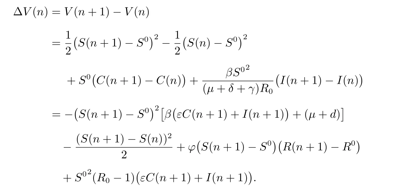
Ifd=0, R0<1, from the last equation of (1), we can get
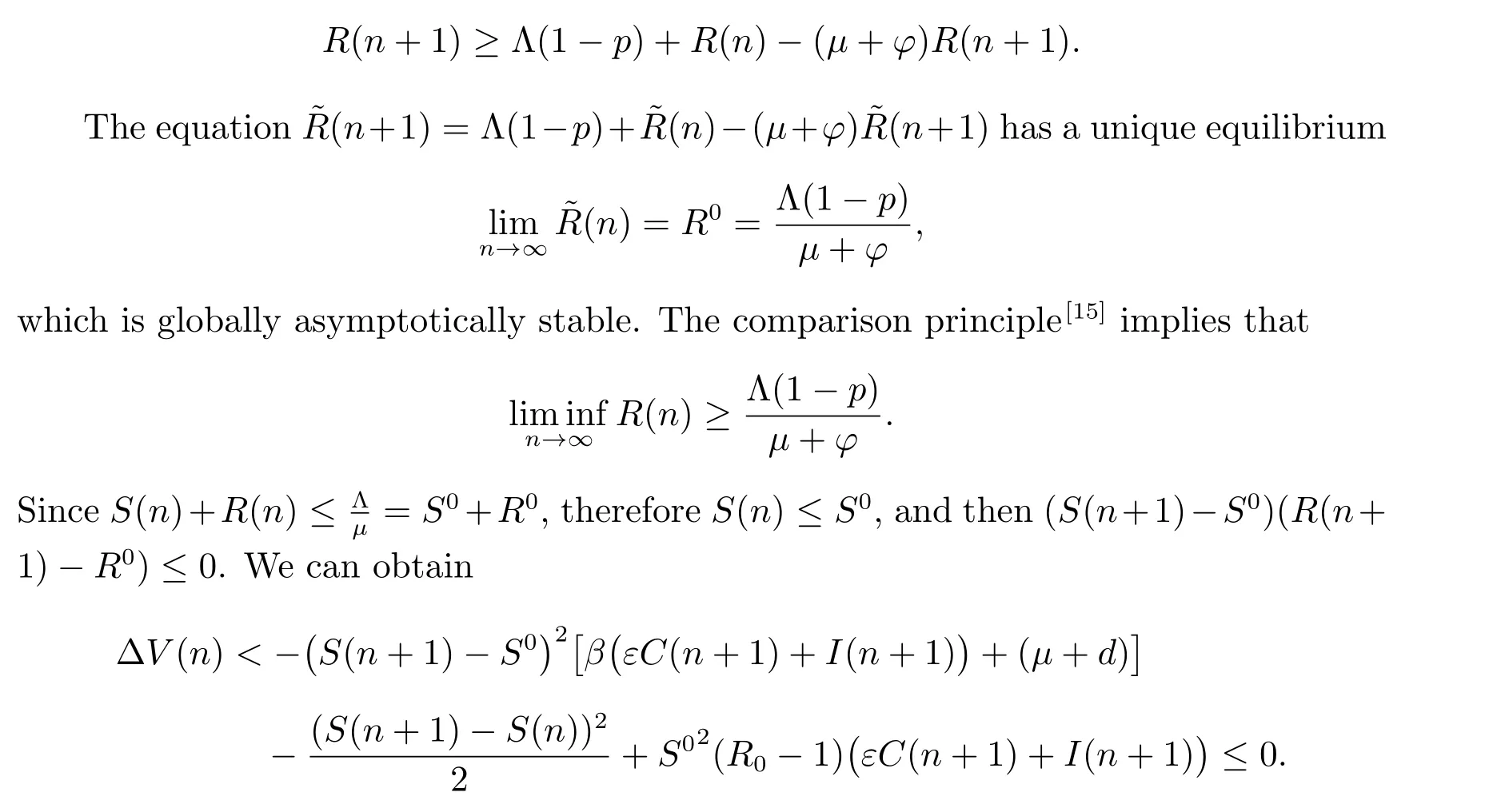

From the above argument, whenR0<1, eitherd=0 orφ=0, we can obtain that ΔV ≤0 in both cases. It is obvious that ΔV= 0 if and only ifS(n) =S0, C(n) =0, I(n) = 0 andR(n) =R0. Based on the LaSalle’s invariance principle[15], we can concludeE0(S0,0,0,R0) is globally asymptotically stable.
Theorem 3 WhenR0>1, eitherd= 0, p= 1, or the other caseφ= 0, the disease will keep persistent in the population.
Proof From Theorem 1, we can obtain that the solution(S(n),C(n),I(n),R(n))of model(1)is positive and bounded. Suppose there exist positive numbersMS, MC, MI,MRsuch that
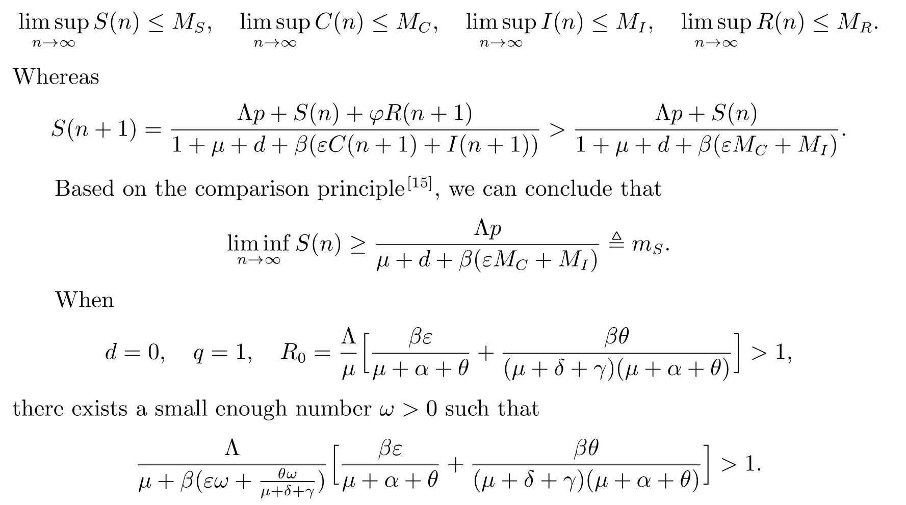
We claim that it is impossible thatC(n)≤ωforn >T1, T1∈N. If the conclusion does not hold. Suppose the contrary, whenn >T1, from the third equation of model(1), we have


Then forn >T2,

Therefore, for any small number

there exists anT3∈N, T3>T2, such that

According to the above inequalities, we define the function

Hence, whenn >T3,
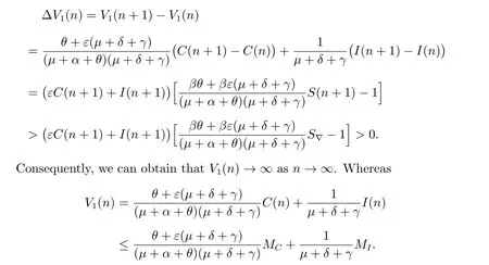
This implies thatV1(n) is bounded, namely, there exists a positive constantT4>T3>0 andV*such thatV1(n)<V*for anyn >T4. This leads to a contradiction.
By the above conclusion, we are left to investigate following two cases:
1) IfC(n)≥ωfor alln >0 sufficiently large. Otherwise;
2)C(n) oscillates aroundωfor alln >0 sufficiently large.
We only need to show that there exists a constant numbermC >0 such thatC(n)≥mCfor allnsufficiently large in the rest part. If the first case holds, similarly,we have lim infn→∞C(n)≥ωand immediately get the conclusion of the theorem.
For another case, we suppose that there are two numbersT5andT6sufficiently large such thatC(T5)≥ωandC(T6)≥ω, butC(n)<ωfor allT5<n <T6.IfT6=T5+2,

Hence

IfT5+2<T6, C(n)<ωfor allT5<n <T6, since ΔV1(n)>0, then we have

Assume that lim infn→∞C(n)=0. Thus,there exists a subsequenceni(limi→∞ni=∞) such that limi→∞C(ni)=0. Since

then

Hence limi→∞V1(ni-1)=0. This leads to a contradiction to the proposition that

Then, we conclude that lim infn→∞C(n)≥mC. From the other equations of model(1), we have

Therefore, the disease will be persistent.
Whenφ=0, the similar argument can be concluded.
4 The stability of the epidemic equilibrium
IfR0>1, apart from the disease-free equilibriumE0, model (1) may admit a unique endemic equilibriumE*(S*,C*,I*,R*), where

Theorem 4 Assume thatR0>1, φ=0,then the endemic equilibriumE*(S*,C*,I*,R*) of model (1) is globally stable.
Proof Let(S(n),C(n),I(n),R(n))be any solution of model(1)with nonnegative initial values. Define the Lyapunov function as

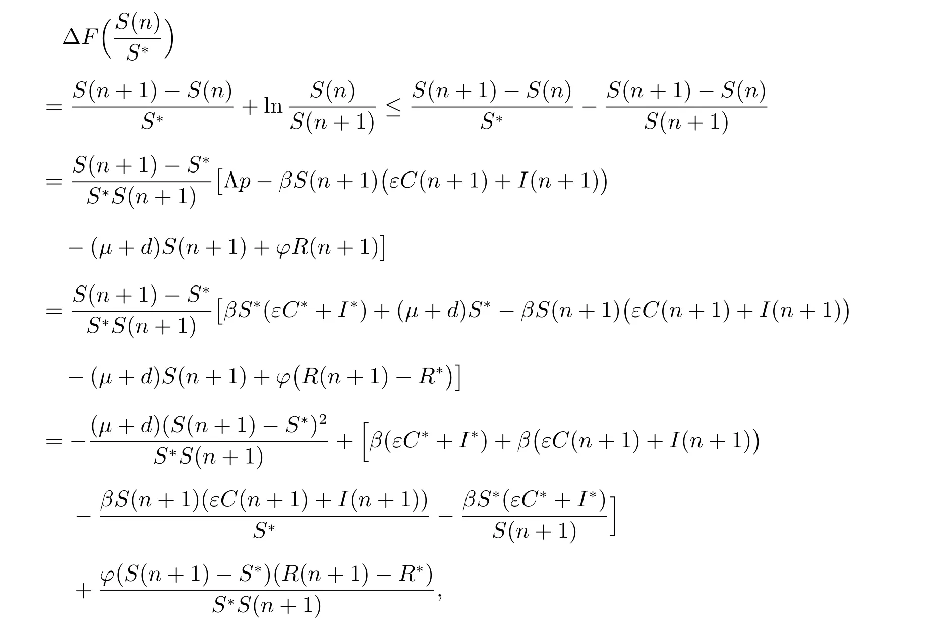
whereF(x)=x-1-lnx,x >0. SinceF(x)=x-1-lnxhas a minimum 0 atx=1,thenF(x)≥0. It is easy to obtain thatU(n) is nonnegative defined with respect to the endemic equilibriumE*. Later we will prove that ΔU(n)=U(n+1)-U(n)≤0.
Since the equilibriumE*(S*,C*,I*,R*) satisfies

we can obtain that

and
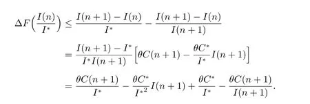
Hence, according to the above inequalities, we have


Whenφ=0, we have

Obviously, ΔU(n)=0 if and only ifS(n+1)=S*,I*C(n+1)=C*I(n+1). This means that

From the first equation of (1), we have that

Using the relations

we can obtain that

Hence

This implies that the infected equilibriumE*is globally asymptotically stable.
5 Numerical simulation
For above discussions,we only obtain sufficient conditions for the global behavior of the equilibrium points. Now we investigate the global behavior of the equilibrium points by numerical simulations to show that the condition is not necessary. For simplicity,we set Λ = 80,p= 0.8,μ= 0.006,ε= 0.7,θ= 0.01,α= 0.005,γ= 0.08,δ= 0.001,d=0.002,φ=0,β=0.000002, then

the condition of Theorem 2 is satisfied. The simulation results show that the diseasefree equilibriumE0(8000,0,0,5333) is globally asymptotically stable, see Figure 1.

Figure 1 R0 =0.6209, φ=0, the global stability of E0
Varying the values ofdandφ, hered=0,φ=0.001, thenR0=0.8574<1, which satisfies the condition of Theorem 2. The simulation results show thatE0(11048,0,0,2285) is globally asymptotically stable, see Figure 2.
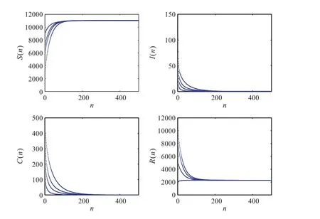
Figure 2 R0 =0.8574, d=0, the global stability of E0
If we continue to change the values ofdandφ,hered=0.002,φ=0.001,thenR0=0.6669<1, the condition of Theorem 2 does not hold. However,E0(8753,0,0,4740) is also globally asymptotically stable, see Figure 3.
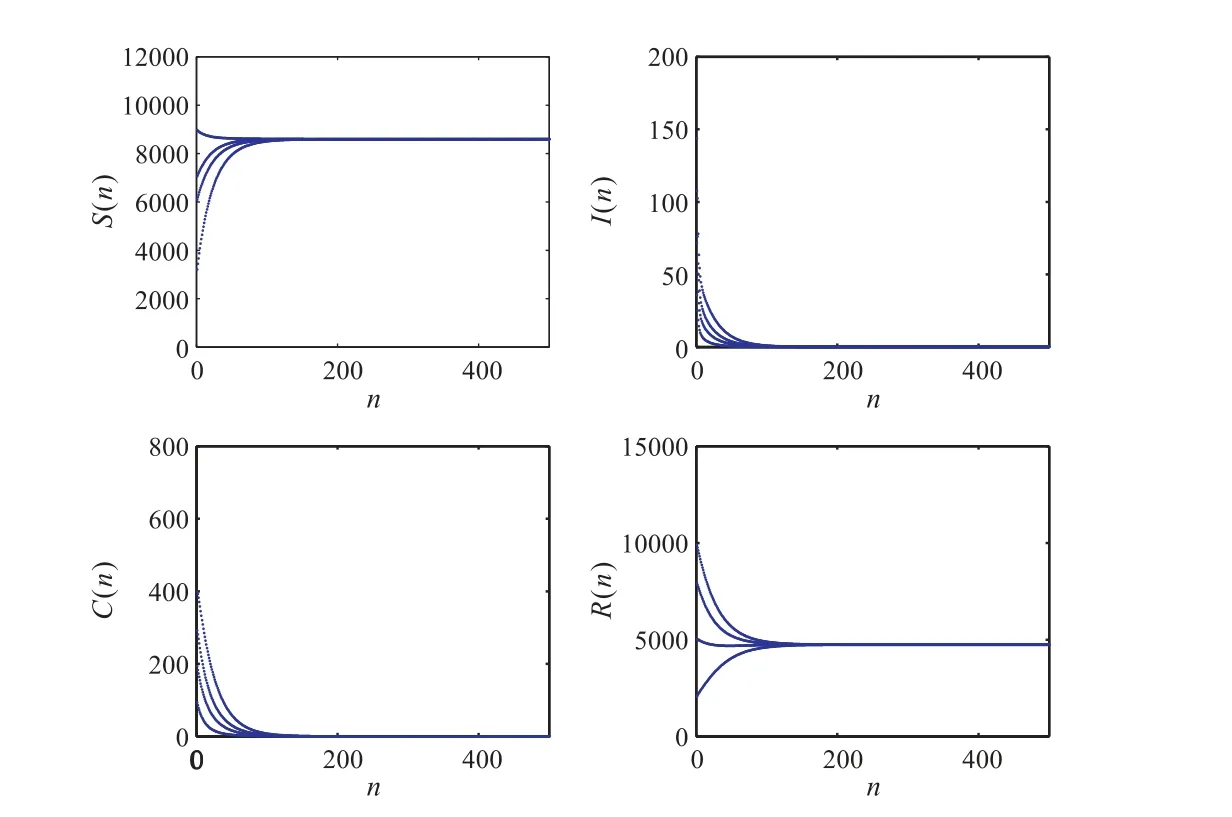
Figure 3 R0 =0.6669, the global stability of E0
With the increase ofβ, if we takeβ= 0.000006,d= 0.002,φ= 0, thenR0=1.8627>1, the condition of Theorem 4 is satisfied. The simulation demonstrates thatE*(4295,1411,162,7438) is globally stable, see Figure 4.
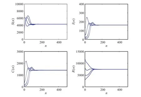
Figure 4 R0 =1.8627,φ=0, the global stability of E*
If we vary the value ofφ, hereφ= 0.001, thenR0= 2.0007>1, the condition of Theorem 4 does not hold. However,E*(4295,1747,201,7057) is also globally stable,see Figure 5. The above numerical simulations show that even if the assumptions of Theorem 2 and Theorem 4 don’t hold,E0may be globally asymptotically stable only whenR0<1, andE*may be globally asymptotically stable only whenR0>1.
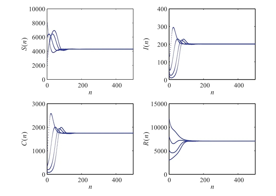
Figure 5 R0 =2.0007, the global stability of E*
6 Discussion
A general discrete Meningococcal Meningitis SCIRS epidemic model is formulated and studied by the backward Euler method in this paper. We obtain sufficient conditions for the global behavior of the disease-free equilibrium and the endemic equilibrium by constructing suitable Lyapunov functions. We make the simulations to demonstrate the stability of the disease-free and endemic equilibrium points of model (1). The simulations show that the equilibrium may be globally stable even if the conditions of Theorem 2 or Theorem 4 do not hold. These observations imply that the conditions in Theorem 2 or Theorem 4 are sufficient but not necessary.

